Which platform should I choose?

Lab 1 — Intro to Python, NumPy, Plotting, and Functions (AI in Earth Science)

0. Working in a Notebook (what to expect)

• This document mixes text cells (like this) and code cells.
• Run cells top → bottom. Variables created above are available below.
• If you re‑run a cell that reassigns a variable, it overwrites the old one.
• Use Shift+Enter to run a cell.
• You can freely edit and re‑run code to experiment.

# Try it: run, edit, re-run
x = 3         # change this
y = 4         # and this
x + y         # the last expression displays automatically

7

Print multiple things: The last expression displays, but if you want more, use print(...).

print("x:", x)
print("y:", y)
print("x + y =", x + y)

x: 3
y: 4
x + y = 7

Note that in coding, an operation like \(z = x + y\) assigns the sum of variables \(x\) and \(y\) to variable \(z\), which is different from the mathematical equality that you’re perhaps more used to (which is denoted by a double equality sign == in python, and many other programming languages). For example, in coding you can have \(x = x+1\). This is of course not a valid mathematical equality for any value of \(x\). In coding it simply means: take whatever value has previously been assigned to \(x\), add 1 to that, and re-assign that value back to \(x\). You can play around with this:

x = 5
x = x + 2
print("x = ", x)

x == x + 2 # Note that this will simply print "False", because x is not equaly to itself plus 2.

x =  7

False

1. Python is interpreted, not compiled (why it matters)

• Interpreted: Python executes statements line‑by‑line at runtime. Easy to explore in notebooks.
• Compiled (C/C++/Fortran): code is translated to machine instructions ahead of time; loops are very fast.

Practical advice in Python for heavy number‑crunching: use NumPy to operate on whole arrays at once.
This style is called vectorization. NumPy runs the heavy math in fast compiled code for you.

# Timing demo: vectorized vs Python loop
import time, math
import numpy as np

n = 1000000  # keep this size reasonable on your machine
xs = np.linspace(0, 100, n)

t0 = time.time()
ys_vec = np.sin(xs) + 0.05*xs**2   # vectorized (fast)
t1 = time.time()
t_vectorized = round(t1 - t0, 4)

ys_loop = []
t2 = time.time()
for v in xs:                        # naive Python loop (slow)
    ys_loop.append(math.sin(v) + 0.05*(v**2))
t3 = time.time()
t_loop = round(t3 - t2, 4)

print("Vectorized (NumPy):", t_vectorized, "s")
print("Loop (pure Python):", t_loop, "s")

speed_up = t_loop/t_vectorized
print("Loop is", round(speed_up), "times faster than vectorized")

Vectorized (NumPy): 0.0287 s
Loop (pure Python): 0.482 s
Loop is 17 times faster than vectorized

The vectorized approach, meaning operations on arrays, is order(s) of magnitude faster because every iteration of a loop needs to be individually translated to machine language when using an interpreter language.

2. Libraries, Imports & Namespaces (np vs numpy)

If you’ve only worked with Matlab before, it’s worth explaining something. Matlab is a large commercial software package and most users will typically install Matlab as a multi-GB application with most functionality included (though one can actually choose to install more/fewer options).

Python, by constrast, is open source and its core functionality only requires around 50-100MB, i.e. tiny. A large world-wide open source community continually adds functionality in the form of libraries/packages like the ones we will use a lot: numpy matplotlib pandas rasterio, which respectively provide tools for linear algebra, plotting, data spreadsheets, and geospatial data.

To use such packages, one usually first has to install those with tools like pip, conda, or mamba. I’m saving you much of that trouble by using google Colab which has most of those packages already installed, though you will see how to install a few more.

One such added features are installed, you can import those functionalities simply as, for example, import numpy. The particular package numpy includes much of the basic functions you would use in Matlab related to linear algebra, as well as functions like sin(), cos(), abs(), exp(), etc. However, plain python also offers several of those functions and those may be implemented slightly differently and perhaps have different inputs and outputs. So a common practice for such packages is to load them as:

• import numpy as np → then call np.sin, np.array, etc.
• import matplotlib.pyplot as plt → then call plt.plot, plt.imshow, etc.

So this clearly tells python to use the function sin of the package numpy and the plotting function plot from matplotlib. In principle, you can use whatever alias you like instead of np and plt, but I usually just stick to those that other people are using so it’s easier to debug etc.

import numpy as np
import matplotlib.pyplot as plt

a = np.array([0, 1, 2, 3], dtype=float)
b = np.sin(a)                       # prefix with np.
print("a:", a)
print("sin(a):", b)

# or we could do
print("Same sine via full name:", numpy_full.sin(a))

a: [0. 1. 2. 3.]
sin(a): [0.         0.84147098 0.90929743 0.14112001]
Same sine via full name: [0.         0.84147098 0.90929743 0.14112001]

3. Python types vs NumPy dtypes

• Python objects have a type: int, float, bool, str, list, tuple, dict, etc.
• NumPy arrays (np.ndarray) store numbers with a dtype (e.g., float64, int32).

Why you care: many libraries (e.g., scikit‑learn) expect numeric arrays of shape (n_samples, n_features) with a float dtype.

p_int = 5
p_float = 5.0
p_list = [1, 2, 3]

print(type(p_int), type(p_float), type(p_list))

arr = np.array([1, 2, 3])          # inferred dtype (usually int64)
print("arr dtype:", arr.dtype)

arr_f = arr.astype(float)          # cast to float
print("arr_f dtype:", arr_f.dtype)

print("Is arr a NumPy array?", isinstance(arr, np.ndarray))

<class 'int'> <class 'float'> <class 'list'>
arr dtype: int64
arr_f dtype: float64
Is arr a NumPy array? True

✅ Try it

• Make a list with both ints and floats. Convert to an array. What dtype do you get?
• Cast to int with .astype(int). What happens to decimals?

# TODO: your experiment
mixed = [1, 2.5, 3, 4.9]
arr_mixed = np.array(mixed)
print("arr_mixed:", arr_mixed, "| dtype:", arr_mixed.dtype)

arr_int = arr_mixed.astype(int)
print("arr_int:", arr_int, "| dtype:", arr_int.dtype)

arr_mixed: [1.  2.5 3.  4.9] | dtype: float64
arr_int: [1 2 3 4] | dtype: int64

4. Arrays vs. math vectors/matrices (and * vs @)

• In math: vector is 1‑D, matrix is 2‑D.
  
• NumPy arrays can be 1‑D, 2‑D, or n‑D.
• Elementwise operations use + - * / and require same shape (or broadcastable shapes).
• Matrix multiplication uses @ (or np.dot), and inner dimensions must match.

A = np.array([[1., 2.],
              [3., 4.]])
B = np.array([[5., 6.],
              [7., 8.]])

print("Elementwise A * B:\n", A * B,"\n")  # Hadamard product       # note how \n adds a new line
print("Matrix A @ B:\n", A @ B,"\n")       # Linear algebra product

print("Shapes:", A.shape, B.shape,"\n")
print("Transpose A.T:\n", A.T,"\n")

Elementwise A * B:
 [[ 5. 12.]
 [21. 32.]] 

Matrix A @ B:
 [[19. 22.]
 [43. 50.]] 

Shapes: (2, 2) (2, 2) 

Transpose A.T:
 [[1. 3.]
 [2. 4.]] 

✅ Mini‑exercise

Create two 3×3 arrays C and D. Print C*D and C@D. Then change a few values and re‑run to see the difference.

# TODO
C = np.arange(9).reshape(3, 3).astype(float)
D = np.ones((3, 3))
print("C*D =\n", C*D)
print("C@D =\n", C@D)

C*D =
 [[0. 1. 2.]
 [3. 4. 5.]
 [6. 7. 8.]]
C@D =
 [[ 3.  3.  3.]
 [12. 12. 12.]
 [21. 21. 21.]]

5. Creating arrays & inspecting shape

Constructors you’ll use constantly: np.array, np.arange, np.linspace, np.zeros, np.ones, np.eye.

v = np.array([0., 1., 2.])
w = np.arange(5)            # 0..4
x = np.linspace(0, 1, 6)    # 6 points from 0 to 1
Z = np.zeros((2,3))
O = np.ones((3,2))
I = np.eye(3)

print("v:", v, "| shape:", v.shape)
print("w:", w)
print("x:", x)
print("Z:\n", Z)
print("O:\n", O)
print("I:\n", I)

v: [0. 1. 2.] | shape: (3,)
w: [0 1 2 3 4]
x: [0.  0.2 0.4 0.6 0.8 1. ]
Z:
 [[0. 0. 0.]
 [0. 0. 0.]]
O:
 [[1. 1.]
 [1. 1.]
 [1. 1.]]
I:
 [[1. 0. 0.]
 [0. 1. 0.]
 [0. 0. 1.]]

6. Reshaping, stacking, and axes

• reshape changes the view of data shape.
• axis tells NumPy which dimension to operate along.
• hstack/vstack or np.concatenate to glue arrays together.

a = np.arange(12)
A = a.reshape(3, 4)      # 3 rows, 4 cols
B = A.T                  # transpose

print("A:\n", A)
print("B = A.T:\n", B)
print("A row sums:", A.sum(axis=1))
print("A col sums:", A.sum(axis=0))

left = np.ones((3,1))
joined = np.hstack([left, A])
print("hstack left|A:\n", joined)

A:
 [[ 0  1  2  3]
 [ 4  5  6  7]
 [ 8  9 10 11]]
B = A.T:
 [[ 0  4  8]
 [ 1  5  9]
 [ 2  6 10]
 [ 3  7 11]]
A row sums: [ 6 22 38]
A col sums: [12 15 18 21]
hstack left|A:
 [[ 1.  0.  1.  2.  3.]
 [ 1.  4.  5.  6.  7.]
 [ 1.  8.  9. 10. 11.]]

7. Indexing & Slicing — the big one

Python is 0‑based (MATLAB is 1‑based). This will likely cause a majority of coding bugs..

Slices exclude the stop. Pattern: start:stop:step.

1‑D examples: - a[0] first element - a[-1] last element - a[:5] indices 0..4 - a[::2] every 2nd - a[::-1] reversed - a[8:2:-2] backwards by 2

2‑D uses A[row, col]. You can slice rows and columns: A[1:3, 0:2].

a = np.arange(10)  # 0..9
print("a:", a)
print("a[0]:", a[0])
print("a[-1]:", a[-1])
print("a[:5]:", a[:5])
print("a[::2]:", a[::2])
print("a[::-1]:", a[::-1])
print("a[8:2:-2]:", a[8:2:-2])

A = np.arange(12).reshape(3, 4)
print("\nA:\n", A)
print("A[1,2]:", A[1,2])
print("A[0,:]:", A[0,:])
print("A[:,0]:", A[:,0])
print("A[0:3,1:3]:\n", A[0:3,1:3])

a: [0 1 2 3 4 5 6 7 8 9]
a[0]: 0
a[-1]: 9
a[:5]: [0 1 2 3 4]
a[::2]: [0 2 4 6 8]
a[::-1]: [9 8 7 6 5 4 3 2 1 0]
a[8:2:-2]: [8 6 4]

A:
 [[ 0  1  2  3]
 [ 4  5  6  7]
 [ 8  9 10 11]]
A[1,2]: 6
A[0,:]: [0 1 2 3]
A[:,0]: [0 4 8]
A[0:3,1:3]:
 [[ 1  2]
 [ 5  6]
 [ 9 10]]

✅ Practice

Given b = np.arange(20): 1) last 5 elements; 2) every 3rd element starting at index 1;
3) reversed copy of the first 10; 4) all but the last two elements (b[:-2]).

# TODO
b = np.arange(20)
print("last 5:", b[-5:])
print("every 3rd from 1:", b[1::3])
print("reverse of first 10:", b[:10][::-1])
print("all but last two:", b[:-2])

last 5: [15 16 17 18 19]
every 3rd from 1: [ 1  4  7 10 13 16 19]
reverse of first 10: [9 8 7 6 5 4 3 2 1 0]
all but last two: [ 0  1  2  3  4  5  6  7  8  9 10 11 12 13 14 15 16 17]

8. Boolean indexing (picking by condition)

Use masks (True/False arrays) to select elements.

x = np.linspace(-3, 3, 13)
mask = x >= 0
print("x:", x)
print("mask:", mask)
print("x[mask]:", x[mask])

# Combine conditions with & | ~
mask2 = (x >= -1) & (x <= 1)
print("x in [-1,1]:", x[mask2])

x: [-3.  -2.5 -2.  -1.5 -1.  -0.5  0.   0.5  1.   1.5  2.   2.5  3. ]
mask: [False False False False False False  True  True  True  True  True  True
  True]
x[mask]: [0.  0.5 1.  1.5 2.  2.5 3. ]
x in [-1,1]: [-1.  -0.5  0.   0.5  1. ]

Optional deeper dive — broadcasting: NumPy can automatically expand compatible shapes.

M = np.arange(12).reshape(3,4)
print("M:\n", M)
col = np.array([[10],[20],[30]])  # shape (3,1)
print("col:\n", col)

print("M + col:\n", M + col)      # col is broadcast across columns, i.e. added to each column

M:
 [[ 0  1  2  3]
 [ 4  5  6  7]
 [ 8  9 10 11]]
col:
 [[10]
 [20]
 [30]]
M + col:
 [[10 11 12 13]
 [24 25 26 27]
 [38 39 40 41]]

9. Slices are often views

A slice often references the same underlying data. Editing a view edits the original.
Use .copy() if you want an independent array.

base = np.arange(10)
view = base[2:7]      # view on base
copy = base[2:7].copy()

view[:] = -1          # modifies the slice (and base)
print("base after editing view:", base)

copy[:] = 99          # does NOT touch base
print("base after editing copy:", base)

base after editing view: [ 0  1 -1 -1 -1 -1 -1  7  8  9]
base after editing copy: [ 0  1 -1 -1 -1 -1 -1  7  8  9]

10. Functions — what & why (math vs coding)

• Math function: a rule mapping inputs to outputs, e.g., ( f(x) = x ).
• Coding function: a reusable block of code you can call with inputs and get outputs. It can combine many operations.

Workflow tip: First write and test a few lines without a function. Once it works, wrap it into a function so you can reuse it.

10.1 Start without a function → then refactor

Goal: convert temperatures from Celsius to Fahrenheit using the rule ( F = 1.8,C + 32 ).

# Step 1: no function
C = np.array([0., 10., 20., 30.])
F = 1.8*C + 32
print("F:", F)

# Step 2: refactor into a function (re-usable)
def c_to_f(c):
    """Convert Celsius to Fahrenheit. Accepts scalars or arrays."""
    c = np.asarray(c)
    return 1.8*c + 32

print("c_to_f([0,10,20,30]):", c_to_f([0,10,20,30]))
print("c_to_f(100):", c_to_f(100))

F: [32. 50. 68. 86.]
c_to_f([0,10,20,30]): [32. 50. 68. 86.]
c_to_f(100): 212.0

Pay attention to the structure of the function, which is a bit different than in Matlab. It starts with def <function_name>(<any nr of inputs): and note the colon as well as the indentation, which needs to be correct. Then, in the tripple quotes you see an explanation of what the function does. THis will be treated just the same as the description of any built-in functions, and you can use for example help(c_to_f) or ? c_to_f to see the help. Finally, the function has to explicitly return one ore more variables. In the example above, the actual computation is included in that return statement, which is nice and short, but you could also make it a bit more explicit like:

def c_to_f(c):
    """Convert Celsius to Fahrenheit. Accepts scalars or arrays."""
    c = np.asarray(c)
    F = 1.8*c + 32
    return F

The most standard way to call a function would of course be something like:

temp_in_C = 30
temp_in_F = c_to_f(temp_in_C)
print("Temp is celcius was", temp_in_C, "which is", temp_in_F, "F.\n")

Note that this function takes 1 input argument and returns 1 output argument. It does not matter what variable names you use for either input or output when calling that function. The variable names in defining the function are just dummies.

# help(c_to_f )
? c_to_f

10.2 Multiple inputs & outputs

Coding functions can take many inputs and return multiple outputs (as a tuple). You can unpack them:

def stats_and_normalize(x):
    """Return (mean, std, z) where z = (x - mean)/std."""
    x = np.asarray(x, dtype=float)
    m = x.mean()
    s = x.std()
    z = (x - m) / s if s != 0 else np.zeros_like(x)
    return m, s, z

data = np.array([1., 2., 3., 4., 5.])
mean, std, z = stats_and_normalize(data)   # unpack
print("mean:", mean, "std:", std)
print("z[:3]:", z[:3])

# If you only need z, you can use dummy names:
_, _, z_only = stats_and_normalize(data)
print("z_only[:3]:", z_only[:3])

mean: 3.0 std: 1.4142135623730951
z[:3]: [-1.41421356 -0.70710678  0.        ]
z_only[:3]: [-1.41421356 -0.70710678  0.        ]

10.3 Scalars vs vectors vs arrays (same function)

Good functions accept scalars or arrays using np.asarray.
Be careful with shape compatibility for elementwise math (e.g., a*b) and matrix multiply (A@B).

def linear(a, x, b):
    """Compute y = a*x + b for scalar/array x."""
    a = np.asarray(a)
    x = np.asarray(x)
    b = np.asarray(b)
    return a*x + b   # elementwise; broadcasting rules apply

print(linear(2.5, np.array([0,1,2]), -1.0))   # vector input
print(linear(2.5, 3.0, -1.0))                 # scalar input

# Example of incompatible shapes for elementwise operations:
try:
    # Broadcastable example (2x1)*(1x3) -> (2x3)
    print(linear(np.ones((2,1)), np.ones((1,3)), 0))

    # Force a failure by making shapes not broadcastable:
    A = np.ones((2,3))
    B = np.ones((4,5))
    C = A * B
except ValueError as e:
    print("ValueError (shape mismatch):", e)

[-1.   1.5  4. ]
6.5
[[1. 1. 1.]
 [1. 1. 1.]]
ValueError (shape mismatch): operands could not be broadcast together with shapes (2,3) (4,5) 

10.4 Checking inputs & raising friendly errors

You can check shapes/types and raise a clear ValueError with a helpful message. != means not-equal-to.

def matmul(A, B):
    """Matrix multiply A @ B with shape checks and clear errors."""
    A = np.asarray(A)
    B = np.asarray(B)
    if A.ndim != 2 or B.ndim != 2:
        raise ValueError(f"matmul expects 2-D arrays, got A.ndim={A.ndim}, B.ndim={B.ndim}")
    if A.shape[1] != B.shape[0]:
        raise ValueError(f"Incompatible shapes for A @ B: {A.shape} and {B.shape} (A.shape[1] must equal B.shape[0])")
    return A @ B

print(matmul([[1,2],[3,4]], [[5],[6]]))
# print(matmul([1,2,3], [4,5,6]))  # uncomment to see the error

[[17]
 [39]]

10.5 Defaults, keywords, docstrings, and help

• Defaults: def f(x, scale=1.0) lets you omit scale or override with a value.
• Keyword arguments improve readability: f(x, scale=2.0).
• Docstrings (triple quotes under def) show up in help(f).

def scale_and_shift(x, scale=1.0, shift=0.0):
    """Return scale*x + shift. Works on scalars or arrays.

    Parameters
    ----------
    x : scalar or array-like
        Input values.
    scale : float, default 1.0
        Multiplicative factor.
    shift : float, default 0.0
        Additive offset.
    """
    x = np.asarray(x, dtype=float)
    return scale*x + shift

print(scale_and_shift([0,1,2], scale=2.0, shift=-1.0))
help(scale_and_shift)

[-1.  1.  3.]
Help on function scale_and_shift in module __main__:

scale_and_shift(x, scale=1.0, shift=0.0)
    Return scale*x + shift. Works on scalars or arrays.
    
    Parameters
    ----------
    x : scalar or array-like
        Input values.
    scale : float, default 1.0
        Multiplicative factor.
    shift : float, default 0.0
        Additive offset.

10.6 Practice: write code, then make it a function

Task: Compute Root‑Mean‑Square Error (RMSE) between predictions yhat and observations y.

1. First, write it inline for the given arrays.
   
2. Then, turn it into a function rmse(yhat, y) that works for scalars and arrays.
   
3. Add an optional argument ignore_nan=False. When True, ignore NaNs safely.

💡 What does ~np.isnan(y) mean? (click to expand)

1. np.isnan(y)
   • Returns a Boolean array: True where elements of y are NaN, False otherwise.
2. ~ (tilde)
   • This is the bitwise NOT operator.
     
   • When applied to Booleans, it flips them: True → False, False → True.

So:

import numpy as np

y = np.array([1.0, np.nan, 3.5])
print(np.isnan(y))   # [False  True False]
print(~np.isnan(y))  # [ True False  True]

::: {#f2c1a874 .cell quarto-private-1='{"key":"colab","value":{"base_uri":"https://localhost:8080/"}}' outputId='bc4c5dd8-fc97-4a6f-c6a7-ce506d103577'}
``` {.python .cell-code}
# Step 1: inline
y = np.array([1.0, 2.0, np.nan, 4.0])
yhat = np.array([1.2, 1.9, 3.0, 3.5])

# TODO: compute rmse inline (once with NaNs, once ignoring NaNs)
mask = ~np.isnan(y) & ~np.isnan(yhat)
rmse_ignore = np.sqrt(np.mean((yhat[mask]-y[mask])**2))
print("Inline RMSE (ignoring NaNs):", rmse_ignore)

# Step 2: wrap into a function
def rmse(yhat, y, ignore_nan=False):
    yhat = np.asarray(yhat, dtype=float)
    y    = np.asarray(y, dtype=float)
    if yhat.shape != y.shape:
        raise ValueError(f"rmse shapes must match: {yhat.shape} vs {y.shape}")
    if ignore_nan:
        m = ~np.isnan(yhat) & ~np.isnan(y)
        if not m.any():
            return np.nan
        diffs = yhat[m] - y[m]
    else:
        diffs = yhat - y
    return np.sqrt(np.mean(diffs**2))

print("Function RMSE:", rmse(yhat, y, ignore_nan=True))

Inline RMSE (ignoring NaNs): 0.31622776601683794
Function RMSE: 0.31622776601683794

:::

11. Vectorization recap

Compute $ y = (x) + 0.1x^2 $ for 1000 points without loops.

x = np.linspace(0, 10, 1000)
y = np.sin(x) + 0.1*x**2  # vectorized
print("y[:5]:", y[:5])

y[:5]: [0.         0.01001986 0.02005876 0.0301157  0.04018966]

12. Plotting with Matplotlib

We’ll make three common plots you’ll reuse later: 1) line plot; 2) scatter; 3) 2‑D image and filled contours.

# Line
x = np.linspace(0, 2*np.pi, 400)
y = np.sin(x) * np.exp(-0.1*x)
plt.figure()
plt.plot(x, y)
plt.title("Damped sine wave")
plt.xlabel("x"); plt.ylabel("y")
plt.show()

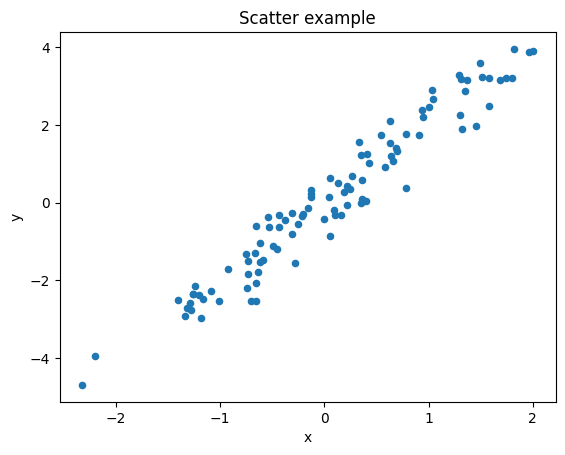
# Scatter
rng = np.random.default_rng(0)
xs = rng.normal(0, 1, 100)
ys = 2*xs + rng.normal(0, 0.5, 100)
plt.figure()
plt.scatter(xs, ys, s=20)
plt.title("Scatter example")
plt.xlabel("x"); plt.ylabel("y")
plt.show()

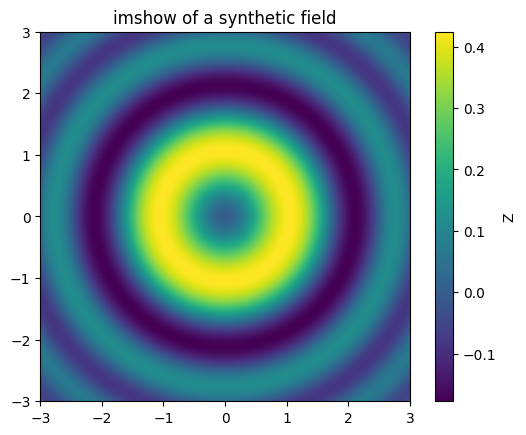
# 2D image & contourf
X = np.linspace(-3, 3, 200)
Y = np.linspace(-3, 3, 200)
XX, YY = np.meshgrid(X, Y)
Z = np.sin(XX**2 + YY**2) / (1 + XX**2 + YY**2)

plt.figure()
plt.imshow(Z, origin="lower", extent=[X.min(), X.max(), Y.min(), Y.max()])
plt.colorbar(label="Z")
plt.title("imshow of a synthetic field")
plt.show()

plt.figure()
cs = plt.contourf(XX, YY, Z, levels=20)
plt.colorbar(cs, label="Z")
plt.title("contourf of a synthetic field")
plt.xlabel("X"); plt.ylabel("Y")
plt.show()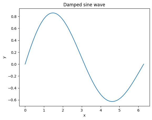

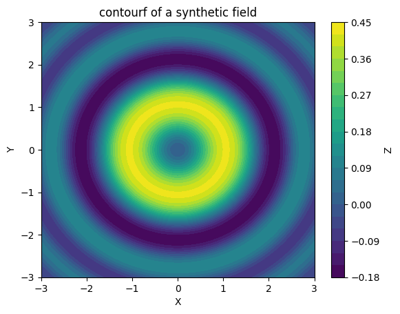
Common plotting pitfalls: - x and y must have the same length for plot/scatter. - In scripts, plt.show() is required to display; in notebooks it’s often automatic but good practice. - Control image axes with origin="lower" and extent=[xmin,xmax,ymin,ymax].

13. Reading errors (tracebacks) — how to debug

When something fails, Python prints a traceback. Scroll to the last lines to find the actual exception (e.g., IndexError, TypeError).

Try each error by uncommenting, read the last line, then fix it.

import numpy as np

A = np.arange(9).reshape(3,3)

# 1) NameError (uncomment to see it)
# print(AA)

# 2) IndexError: valid rows are 0..2
# print(A[3,0])

# 3) TypeError: list vs array elementwise
# L = [1, 2, 3]
# print(L * L)  # not elementwise!

print("Done (no errors because they're commented out).")

Done (no errors because they're commented out).

General tips: 1. Read the last line of the error. 2. Print shapes (.shape) and types (type(x), arr.dtype). 3. Prefer vectorized NumPy over Python loops. 4. Beware slices as views; use .copy() when needed. 5. Avoid shadowing names like np, plt, or sum.

14. Common beginner pitfalls (and how to avoid them)

• Off‑by‑one from 0‑based indexing and slice stop being excluded.
• * vs @: elementwise vs matrix multiply.
• Shape mismatches: check A.shape, B.shape (for A @ B, inner dims must match).
• Lists don’t do numeric math; convert with np.array.
• / returns float; use // for integer floor division.
• Slices return views; use .copy() for independent arrays.
• Attributes vs methods: arr.shape (no ()), but arr.mean() does need ().
• Namespace collisions: avoid from numpy import * and avoid naming variables np, plt, list, sum, etc.

15. Quick self‑tests (run; no assertion errors means you’re good)

import numpy as np

# Slicing
a = np.arange(10)
assert (a[:5] == np.array([0,1,2,3,4])).all()
assert (a[-3:] == np.array([7,8,9])).all()

# Elementwise vs matmul shapes
A = np.array([[1,2],[3,4]])
B = np.array([[5,6],[7,8]])
assert (A*B).shape == (2,2)
assert (A@B).shape == (2,2)

# Dtype conversion
arr = np.array([1,2,3])
arrf = arr.astype(float)
assert arrf.dtype.kind == 'f'

# Boolean mask
x = np.array([-1, 0, 1, 2])
mask = x >= 0
assert (x[mask] == np.array([0,1,2])).all()

# Functions section (simple checks)
def _rmse(yhat, y, ignore_nan=False):
    yhat = np.asarray(yhat, dtype=float)
    y    = np.asarray(y, dtype=float)
    if ignore_nan:
        m = ~np.isnan(yhat) & ~np.isnan(y)
        if not m.any(): return np.nan
        yhat, y = yhat[m], y[m]
    return np.sqrt(np.mean((yhat - y)**2))

assert np.isclose(_rmse([1,2,3],[1,2,3]), 0.0)
assert np.isfinite(_rmse([1,2,np.nan],[1,2,3], ignore_nan=True))

print("All quick checks passed ✅")

All quick checks passed ✅

16. Next steps

• Keep this open during the semester as a cheat sheet.
• As you code: print shapes and types early and often.
• Prefer vectorized NumPy over plain Python loops for numerics.
• When stuck, read the last lines of the traceback, reduce to a small example, and iterate.

---

📖 Next module: Module 2: Linear Regression