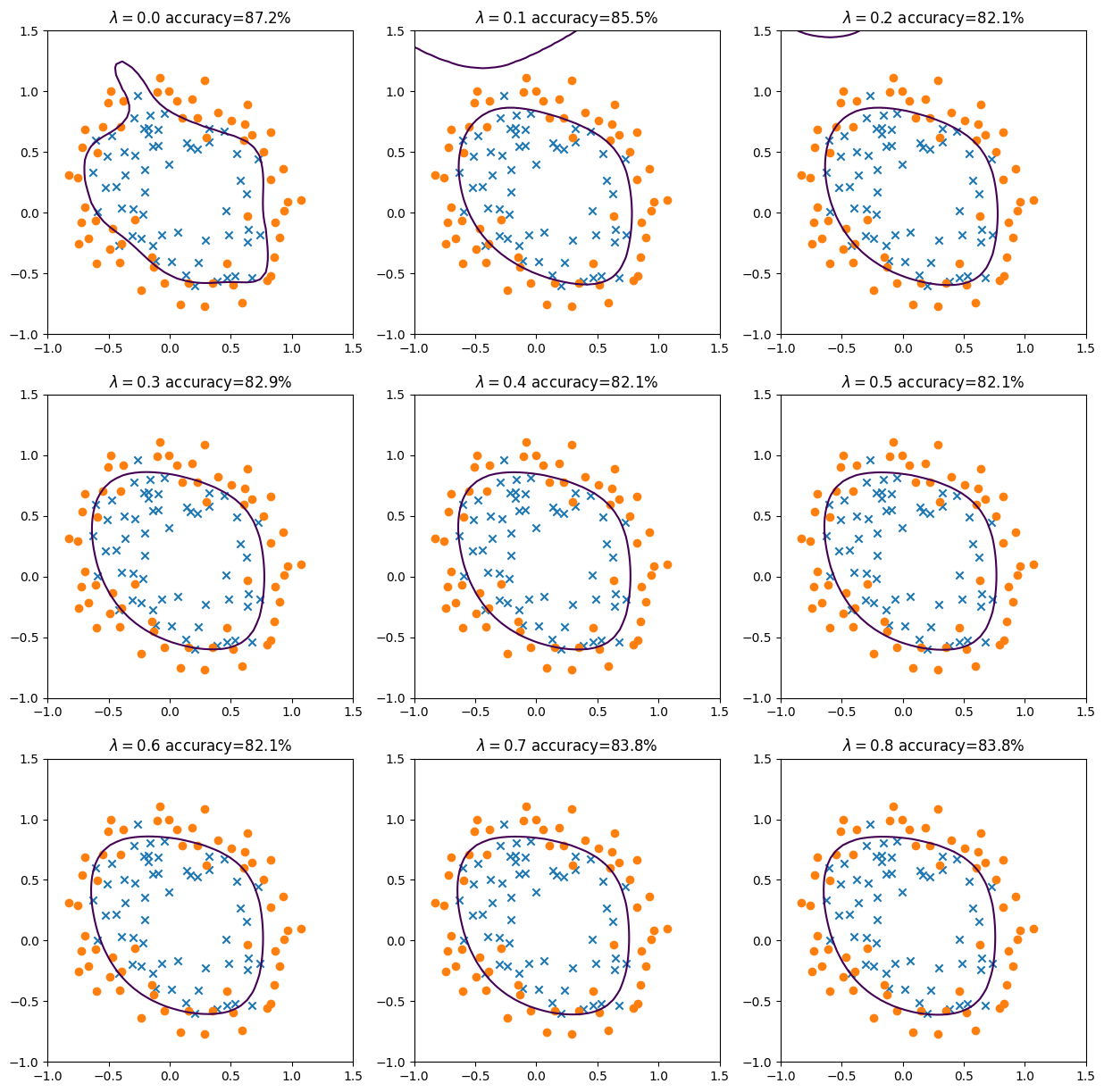
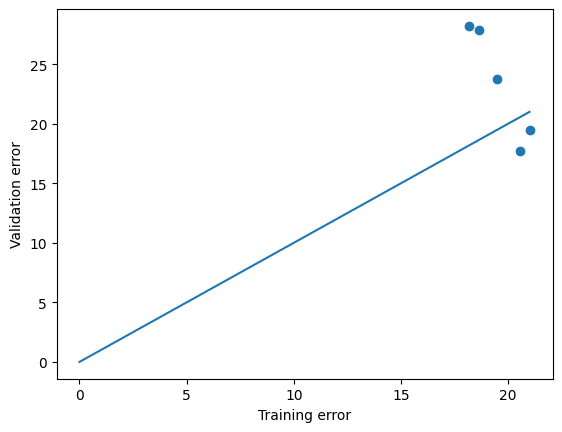
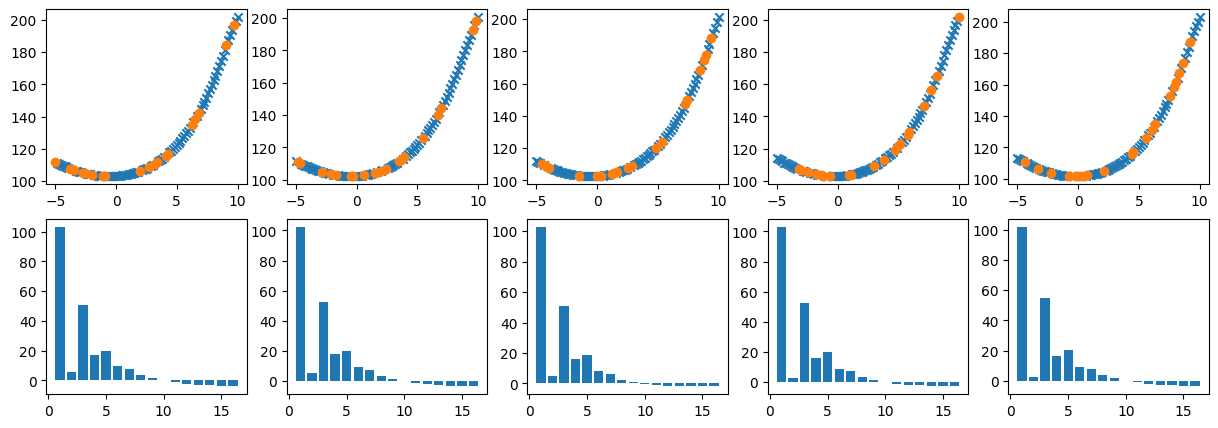
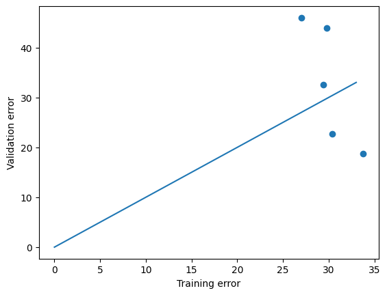
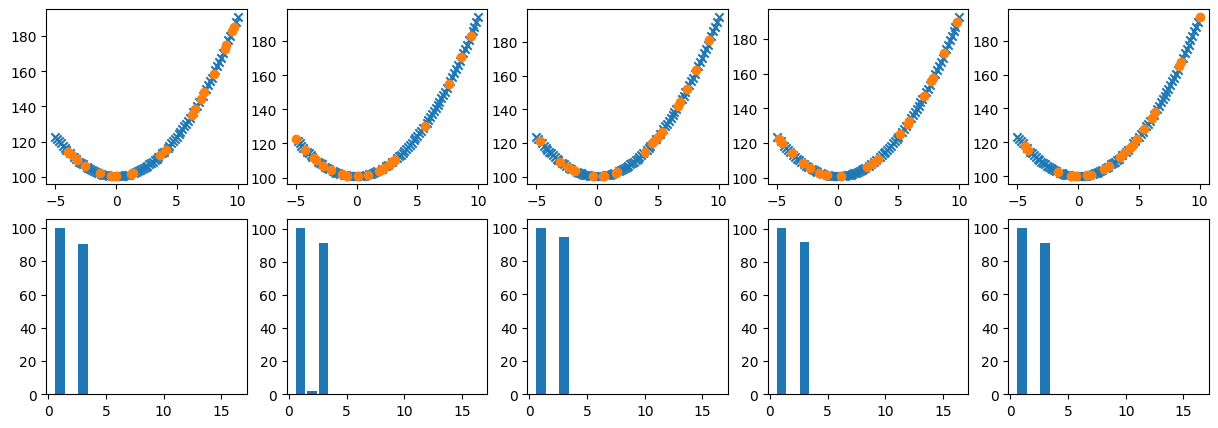
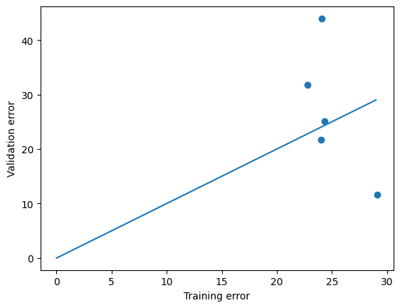
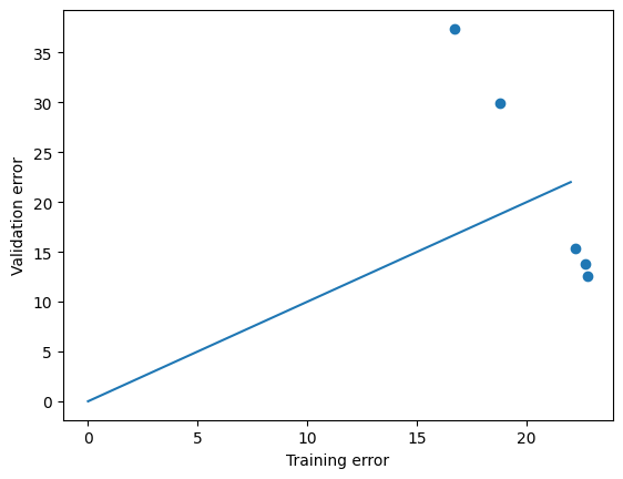
# Illustrative plots:
fig = plt.figure(figsize=(15,40))
nr_fits = 101
m = np.shape(y)[0]
x1_range = x
x2_range = x**2
x_1 = x1_range
x_2 = x2_range
LSerror = np.zeros([nr_fits,nr_fits])
# Try all combinations of theta_1 and theta_2 between -2 and 2 in 101 steps
thetas1_rng = np.linspace(-2,2,nr_fits)
thetas2_rng = np.linspace(-2,2,nr_fits)
theta1, theta2 = np.meshgrid(thetas1_rng,thetas2_rng)
LassoError = np.zeros([nr_fits,nr_fits])
RidgeError = np.zeros([nr_fits,nr_fits])
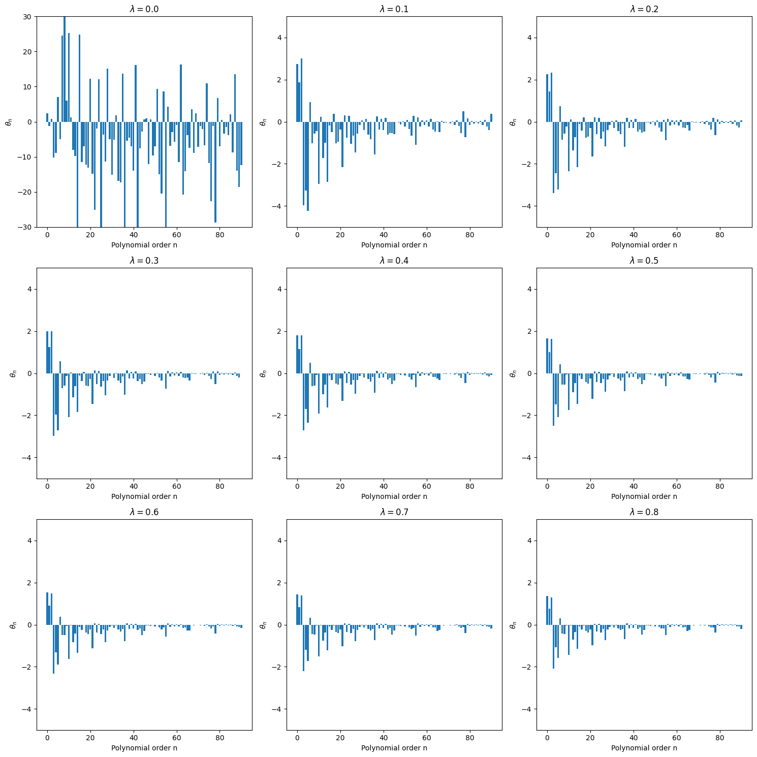
savelassos = np.zeros([8,3]) # 8 different regularization strenghts
saveridges = np.zeros([8,3])
for k in range(1,8):
lambda_reg = k*0.01
# Compute full grid of errors:
for i in range(nr_fits):
for j in range(nr_fits):
y_pred = theta1[i,j] * x1_range + theta2[i,j] * x2_range
LSerror[i,j] = mean_squared_error(y_pred,y)
LassoError[i,j] = lambda_reg * ( np.abs(theta1[i,j]) + np.abs(theta2[i,j]))
RidgeError[i,j] = lambda_reg * ( theta1[i,j]**2 + theta2[i,j]**2)
# Minimum least-squares, Lasso, and Ridge errors and corresponding best fit theta:
LSerrormin = np.min(LSerror)
min_ind = np.where(LSerror==LSerrormin)
besttheta1 = theta1[min_ind[0],min_ind[1]].item()
besttheta2 = theta2[min_ind[0],min_ind[1]].item()
print(k, min_ind, "lambda = ", lambda_reg,
"Best least squared theta:", besttheta1,besttheta2,
"with error:", LSerrormin )
lasserror = LSerror+LassoError
Lassoerrormin = np.min(lasserror)
min_ind = np.where(lasserror==Lassoerrormin)
besttheta1_lasso = theta1[min_ind[0],min_ind[1]].item()
besttheta2_lasso = theta2[min_ind[0],min_ind[1]].item()
savelassos[k-1,0] = lambda_reg
savelassos[k-1,1] = besttheta1_lasso
savelassos[k-1,2] = besttheta2_lasso
print(k, min_ind,"lambda = ", lambda_reg,
"Best Lasso theta:", besttheta1_lasso,besttheta2_lasso,
"with error:", Lassoerrormin )
ridgeerror = LSerror+RidgeError
Ridgeerrormin = np.min(ridgeerror)
min_ind = np.where(ridgeerror==Ridgeerrormin)
besttheta1_ridge = theta1[min_ind[0],min_ind[1]].item()
besttheta2_ridge = theta2[min_ind[0],min_ind[1]].item()
saveridges[k-1,0] = lambda_reg
saveridges[k-1,1] = besttheta1_ridge
saveridges[k-1,2] = besttheta2_ridge
print(k, min_ind,"lambda = ", lambda_reg,
"Best Ridge theta:", besttheta1_ridge,besttheta2_ridge,
"with error:", Ridgeerrormin )
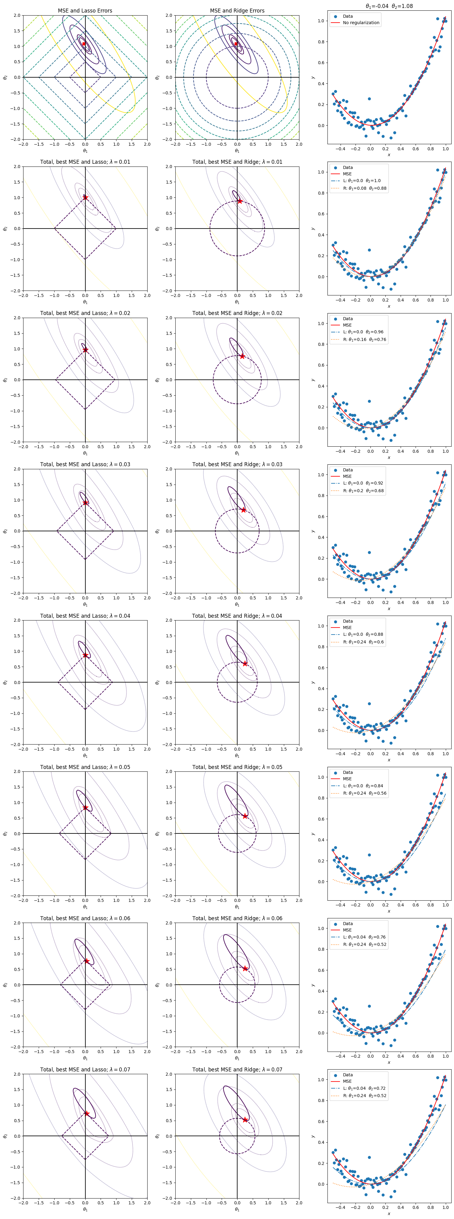
if(k==1):
plt.subplot(8,3,1)
toterr = LSerror
plt.contour(theta1, theta2, toterr,
levels=[1.5*np.min(toterr),2*np.min(toterr),
5*np.min(toterr),10*np.min(toterr),
50*np.min(toterr)])
plt.contour(theta1, theta2, LassoError, linestyles='dashed')
plt.scatter(besttheta1,besttheta2,marker='x',color='red',linewidths=4)
plt.xlabel(r'$\theta_1$')
plt.ylabel(r'$\theta_2$')
plt.title('MSE and Lasso Errors')
plt.gca().set_aspect('equal', adjustable='box')
plt.axhline(y=0, color='k')
plt.axvline(x=0, color='k')
plt.subplot(8,3,2)
toterr = LSerror
plt.contour(theta1, theta2, toterr,
levels=[1.5*np.min(toterr),2*np.min(toterr),
5*np.min(toterr),10*np.min(toterr),
50*np.min(toterr)])
plt.contour(theta1, theta2, RidgeError,linestyles='dashed')
plt.scatter(besttheta1,besttheta2,marker='x',color='red',linewidths=4)
plt.xlabel(r'$\theta_1$')
plt.ylabel(r'$\theta_2$')
plt.title('MSE and Ridge Errors')
plt.gca().set_aspect('equal', adjustable='box')
plt.axhline(y=0, color='k')
plt.axvline(x=0, color='k')
plt.subplot(8,3,3)
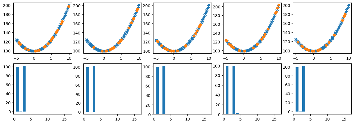
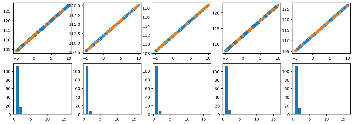
thetitle = r'$\theta_1$='+str(np.round(besttheta1,2))+' '+r'$\theta_2$='+str(np.round(besttheta2,2))
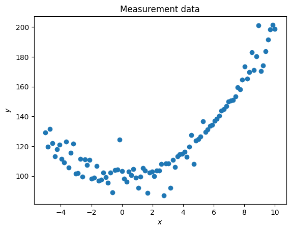
plt.scatter(x1_range,y)
y_pred = besttheta1*x1_range + besttheta2* x2_range
plt.plot(x1_range, y_pred,'r-')
plt.legend(['Data', 'No regularization'])
plt.xlabel(r'$x$')
plt.ylabel(r'$y$')
plt.title(thetitle)
l = k*3 + 1
plt.subplot(8,3,l)
print("Plotting panels", l, 'for regularization param', k, lambda_reg)
toterr = LSerror+LassoError
plt.contour(theta1, theta2, toterr,
levels=[1.5*np.min(toterr),2*np.min(toterr),
5*np.min(toterr),10*np.min(toterr),
50*np.min(toterr)],linestyles='dotted',linewidths=1)
plt.scatter(besttheta1_lasso,besttheta2_lasso,marker='*',color='red',s=200)
minlassoerr = lambda_reg*(np.abs(besttheta1_lasso) + np.abs(besttheta2_lasso))
plt.contour(theta1, theta2, LassoError, levels=[minlassoerr],linestyles='dashed')
minlLEerr = mean_squared_error(besttheta1_lasso * x_1 + besttheta2_lasso * x_2,y)
plt.contour(theta1, theta2, LSerror, levels=[minlLEerr])
plt.xlabel(r'$\theta_1$')
plt.ylabel(r'$\theta_2$')
plt.title('Total, best MSE and Lasso; '+r'$\lambda=$'+str(round(lambda_reg,2)))
plt.gca().set_aspect('equal', adjustable='box')
plt.axhline(y=0, color='k')
plt.axvline(x=0, color='k')
plt.subplot(8,3,l+1)
print("Plotting panels", l+1, 'for regularization param', k, lambda_reg)
toterr = LSerror+RidgeError
plt.contour(theta1, theta2, toterr,
levels=[1.5*np.min(toterr),2*np.min(toterr),
5*np.min(toterr),10*np.min(toterr),
50*np.min(toterr)],linestyles='dotted',linewidths=1)
plt.scatter(besttheta1_ridge,besttheta2_ridge,marker='*',color='red',s=200)
minridgeerr = lambda_reg *( besttheta1_ridge**2 + besttheta2_ridge**2)
plt.contour(theta1, theta2, RidgeError, levels=[minridgeerr],linestyles='dashed')
minlLEerr = mean_squared_error(besttheta1_ridge * x_1 + besttheta2_ridge * x_2,y)
plt.contour(theta1, theta2, LSerror, levels=[minlLEerr])
plt.axhline(y=0, color='k')
plt.axvline(x=0, color='k')
plt.xlabel(r'$\theta_1$')
plt.ylabel(r'$\theta_2$')
plt.title('Total, best MSE and Ridge; '+r'$\lambda=$'+str(round(lambda_reg,2)))
plt.gca().set_aspect('equal', adjustable='box')
plt.subplot(8,3,l+2)
plt.scatter(x1_range,y)
y_pred = besttheta1*x1_range + besttheta2* x2_range
plt.plot(x1_range, y_pred,'r-')
y_pred = besttheta1_lasso*x1_range + besttheta2_lasso* x2_range
plt.plot(x1_range, y_pred,'-.')
y_pred = besttheta1_ridge*x1_range + besttheta2_ridge* x2_range
plt.plot(x1_range, y_pred,':')
lasso_label = 'L: ' + r'$\theta_1$='+str(np.round(besttheta1_lasso,2))+' '+r'$\theta_2$='+str(np.round(besttheta2_lasso,2))
ridge_label = 'R: ' + r'$\theta_1$='+str(np.round(besttheta1_ridge,2))+' '+r'$\theta_2$='+str(np.round(besttheta2_ridge,2))
plt.legend([ "Data", 'MSE', lasso_label,ridge_label])
plt.xlabel(r'$x$')
plt.ylabel(r'$y$')
fig.tight_layout()
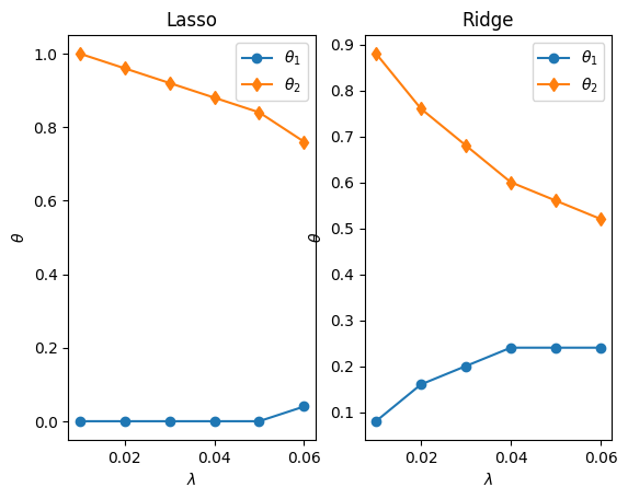
plt.figure()
plt.subplot(1,2,1)
plt.plot(savelassos[:-2,0],savelassos[:-2,1],'-o')
plt.plot(savelassos[:-2,0],savelassos[:-2,2],'-d')
plt.xlabel(r'$\lambda$')
plt.ylabel(r'$\theta$')
plt.legend([r'$\theta_1$',r'$\theta_2$'])
plt.title('Lasso')
plt.subplot(1,2,2)
plt.plot(saveridges[:-2,0],saveridges[:-2,1],'-o')
plt.plot(saveridges[:-2,0],saveridges[:-2,2],'-d')
plt.xlabel(r'$\lambda$')
plt.ylabel(r'$\theta$')
plt.legend([r'$\theta_1$',r'$\theta_2$'])
plt.title('Ridge')

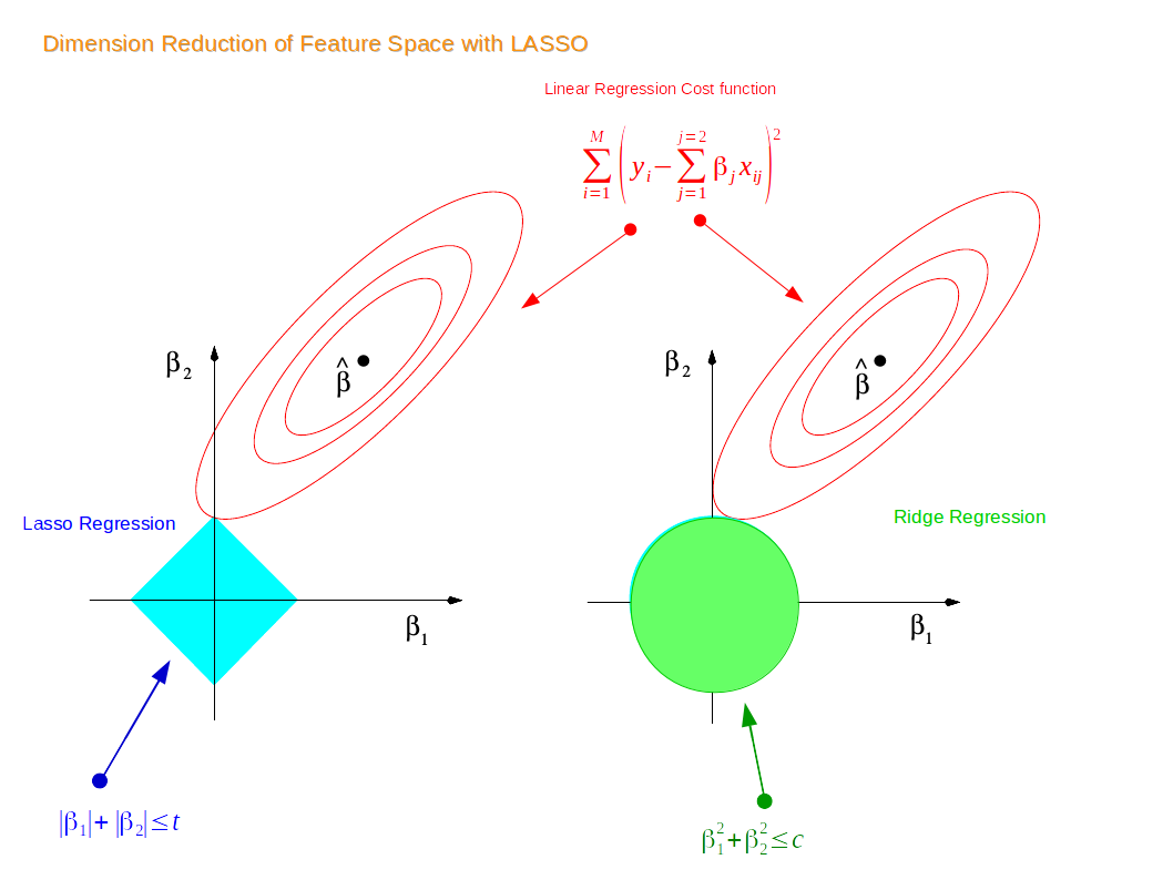 from https://miro.medium.com/max/2116/1*Jd03Hyt2bpEv1r7UijLlpg.png A super-detailed discussion can also be found here: https://www.coursera.org/lecture/ml-regression/deriving-the-lasso-coordinate-descent-update-6OLyn , but it uses yet another alternative to gradient descent: coordinate descent. In coordinate descent, fitting is essentially done for one coordinate