Which platform should I choose?

✏️ After this lecture, try the Practice exercise

Univariate Linear Logistic Regression for Binary Classification Problem

In this Unit we introduce the concept of logistic, as opposed to numerical, regression. In numerical regression, we fit continuous variables. The target (\(y\)) is a continous function of the (linear or nonlinear) features (\(x\)). In logistic regression, the features may be either continuous or discrete (often a mixture of discrete and continuous features), but the target is discrete.

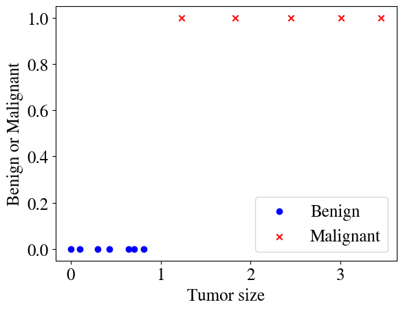
As with numerical regression, we can have either a single (univariate) feature, or multiple (multivariate) features, but we only have one target. The target can only take on a fixed number of discrete values, which represent categories or classes. Logistic regressions are classification schemes. In the simplest case, which we’ll look at first, we only have two categories, and this is called a binary classification scheme. As an example, we could categorize whether an email is spam or not spam, which we can label with 0 for not-spam and 1 for spam (or the other way around; that doesn’t matter). As a very simplistic spam filter, we could have a single feature such as the fraction of letters in the email that are capitalized and then train a binary classification model on a large number of emails to figure out (fit) what fraction of capital letters corresponds to emails that a user flags as spam (\(y=1\)) or not spam (\(y=0\)). As another (somewhat macabre) example, which we’ll use below, a doctor could measure tumors on a large number of patients and determine based on the tumor size whether it is benign (\(y=0\)) or malignant (\(y=1\)).

We will also consider the next level of complexity in which the target is still binary (\(y=0\) or \(y=1\)), but depends on multiple features. As before, for visualization reasons we will only consider here examples that depend on two features \(x_1\) and \(x_2\).

And finally, we will consider multiclass classification schemes with any number of categories. This is a common objective in image recognition. The example we’ll consider in the Lab is to recognize handwritten numbers and categorize images into \(0, 1, \ldots, 9\), i.e. 10 categories. You encounter similar multi-category classification schemes every day nowadays, which automatically detect which of your friends and family show up in your pictures.

Load libraries

Note that I just load a bunch of libraries that I often end up using; not all of these are necessarily used in this notebook.

from __future__ import division
import numpy as np
import matplotlib.pyplot as plt

# from matplotlib import animation
from IPython import display
import scipy.sparse as sp
import scipy.sparse.linalg
from scipy.linalg import solve_banded
from scipy import optimize

import time

%matplotlib inline
# %matplotlib notebook
from IPython.core.debugger import set_trace
plt.rcParams['figure.dpi'] = 100
plt.rcParams.update({'font.size': 18, 'font.family': 'STIXGeneral', 'mathtext.fontset': 'stix'})
# plt.rcParams['text.usetex'] = True
import pandas as pd

from sklearn.metrics import mean_absolute_error,mean_squared_error
from sklearn.model_selection import train_test_split
# To insert values for missing data
from sklearn.impute import SimpleImputer
# To translate text cell values into numerical labels
from sklearn.preprocessing import LabelEncoder
from sklearn.utils import shuffle
##################
from sklearn.linear_model import LinearRegression, Ridge, Lasso
##################
# Decision trees:
from sklearn.tree import DecisionTreeRegressor
from sklearn.ensemble import RandomForestRegressor
from sklearn.tree import export_graphviz
#Neural networks:
from sklearn.model_selection import cross_val_score
from sklearn.model_selection import KFold
from sklearn.preprocessing import StandardScaler
from sklearn.pipeline import Pipeline

# from keras.callbacks import ModelCheckpoint
# from keras.models import Sequential
# from keras.layers import Dense
# from keras.wrappers.scikit_learn import KerasRegressor

from mpl_toolkits.mplot3d import Axes3D  # noqa: F401 unused import
# State of the art Extreme Gradient Booster:
from xgboost import XGBRegressor
import requests

import warnings
warnings.filterwarnings("ignore", category=DeprecationWarning)


small = 0.0000000001

Generate example data set

As in every notebook before, let’s start by generating some illustrative synthetic data. Our feature is tumor size in some unspecified unit, and the target is to predict whether a tumor is benign or malignant. A supervised machine learning algorithm will be trained on some labeled data (i.e. a number of cases where a doctor would have measured a tumor and determined whether it was benign or not). Our objective is to fit such data, and then the fitted model can be used to predict the outcome of future data (i.e., other future measurements of tumor sizes).

These first examples may seem overly simplified and perhaps not very interesting, but fear not, I don’t think I’m wasting your time or insulting your intelligence; the key concepts illustrated by these examples can be extended in surprisingly straightforwards ways to highly complex non-linear, multi-class, logistical regression categorization schemes, and even as you will see to deep neural network machine learning algorithms.

With that said, here’s our synthetic data for the first example:

x = np.array([0,0.1, 0.3, 0.43, 0.64, 0.70, 0.81, 1.23, 1.83,2.45, 3.01, 3.45])
y = np.array([0,0,0,0,0,0,0,1,1,1,1,1])

# Plotting:
plt.scatter(x[:7],y[:7],color='blue',marker='o', label='Benign')
plt.scatter(x[7:],y[7:],color='red',marker='x', label='Malignant')
plt.legend(loc='lower right')

plt.xlabel('Tumor size')
plt.ylabel('Benign or Malignant')


Y = y
x = x[:,None]
y = y[:,None]

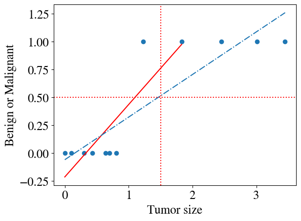
It is probably fairly obvious that applying a linear regression model to this type of data does not make a lot of sense. Below, two such fits are shown. The first one fits all but the last three points. For that fit, one could say that when the fitted \(\tilde{y}(x)\ge0.5\) we assume the tumor is malignant and when \(\tilde{y}<0.5\) it is benign. But the example also shows that if a few more tumors had been measured with larger sizes, the fit would have been completely different (the dash-dotted line) and the \(\tilde{y}(x)\ge0.5\) criteria no longer correctly predicts which tumors are benign or not. Also note that such linear hypotheses will always predict \(y<0\) and \(y>1\) for certain values of \(x\), which is not possible for these types of binary classification problems (values \(0<y<1\) are not that problematic and can be interpretted as probabilities of being 1 or 0, i.e. a a value \(y=0.7\) could suggest a 70% probability of being malignant).

plt.scatter(x,y)

# don't fit to last 3 points
my_linear_regression_model = LinearRegression().fit(x[:-3], y[:-3])
y_pred = my_linear_regression_model.predict(x[:-3])

plt.plot(x[:-3],y_pred,'r')

# fit to all points
my_linear_regression_model = LinearRegression().fit(x, y)
y_pred = my_linear_regression_model.predict(x)

plt.plot(x,y_pred, linestyle='-.')
plt.axvline(x=1.5, color='r', linestyle=':')
plt.axhline(y=0.5, color='r', linestyle=':');

plt.xlabel('Tumor size')
plt.ylabel('Benign or Malignant');

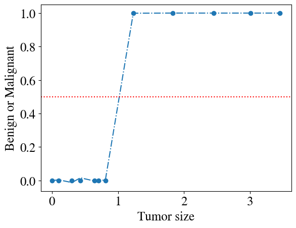
Having paid attention in the previous modules, you may think that we can easily fix this problem by considering some higher-order polynomial hypothesis instead! Indeed, any function no matter how complicated can be fitted by a polynomial of sufficiently high order. Below you see an example for a 9th order polynomial (code copy-pasted from previous module) and the fit is pretty good. Increase the order to 10 or more and the fit is excellent. However, try this (see if you can do it): do the fitting for all but the last measurement point (i.e. consider all measurements except just one as your training data, and just the last point as a validation data point). Just as in the last module, you’ll see that such a point outside the range of the training data cannot be predicted by this high-order polynomial, which will completely explode in some wrong direction (to the point where you can’t really see the actuall fitted points anymore, which is why I’m not already plotting it below).

plt.scatter(x,y)
# fit to all points
poly_order = 9
features = np.zeros([len(x),poly_order])

for i in range(poly_order):
    features[:,i] = x[:,0]**(i+1)

my_linear_regression_model = LinearRegression().fit(features, y)
y_pred = my_linear_regression_model.predict(features)
plt.plot(x,y_pred, linestyle='-.')

plt.axhline(y=0.5, color='r', linestyle=':')

plt.xlabel('Tumor size')
plt.ylabel('Benign or Malignant')

Text(0, 0.5, 'Benign or Malignant')

Sigmoid function

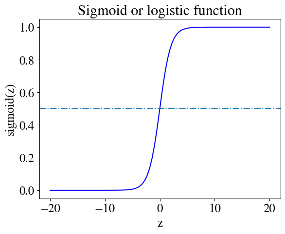
The take-away point so far is that it doesn’t make sense to use polynomials (including linear) to fit a dependent variable \(y\) that can only take on two distinct values: 0 and 1. There is, however, another function that is beautifully well-suited for this problem. That function is called the sigmoid or (synonymously) logistic function, explaining why these categorization schemes are called logistic regressions. The sigmoid function is defined as:

\(g(z) = \frac{1}{1+\mathrm{e}^{-z}}\).

Below we define a python function to compute the sigmoid and plot it, which shows why this is obviously a useful function to use for a binary classification scheme.

def sigmoid(z):
  return 1/(1 + np.exp(-z))

plt.figure()
z = np.linspace(-20,20,100)
plt.plot(z,sigmoid(z), 'b')
plt.xlabel('z')
plt.ylabel('sigmoid(z)')
plt.title('Sigmoid or logistic function')
plt.axhline(y=0.5,linestyle='-.');

The figure shows that the function is centered around \(z=0\) where it takes on the value \(g(z)=0.5\). For values \(z\) not much larger than \(z=0\), \(g(z)\) quickly asymptotes to \(g(z)=1\) for all \(z\) somewhat larger than zero, whereas \(g(z)=0\) for all \(z\) somewhat below zero.

Just like any other function (like a sine, a quadratic function, or any other example), we can shift the function left or right and change the slope. Specifically, in this one-feature (\(x\)) example, we can write:

\(z = \theta_0 + \theta_1 x\)

or, adding a bias feature \(x_0=1\) with \(x_1=x\), defining a vector of the fitting parameters \(\vec{\theta} = [\theta_0, \theta_1]^T\) (should be a column vector) and feature array \(\mathbf{X}\), we have

\(z = \mathbf{X}\cdot \vec{\theta}\)

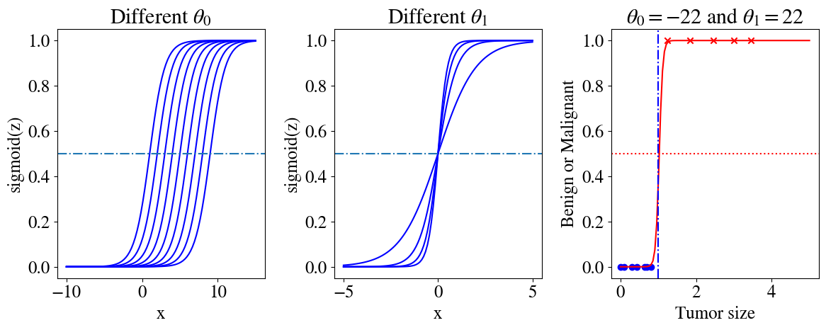
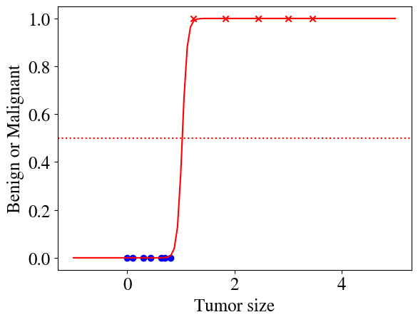
The code below generates three illustrations of sigmoid functions. The first figure those how the sigmoid function can be shifted horizontally by varying \(\theta_0\), the second shows how the slope (in the narrow region where \(g(z)\) is not 0 or 1) can be tuned by \(\theta_1\). The final panel shows how \(g(z)\) with \(z = \theta_0 + \theta_1 x\), together with \(\theta_0=-22\) and \(\theta_1=22\) can perfectly match our measurements.

plt.figure(figsize=(12,5))

plt.subplot(1,3,1)
feature = np.linspace(-10,15,100)

for i in range(1,10):
  z = -i + feature
  plt.plot(feature,sigmoid(z), 'b')

plt.xlabel('x')
plt.ylabel('sigmoid(z)')
plt.title('Different '+r'$\theta_0$')
plt.axhline(y=0.5,linestyle='-.')


feature = np.linspace(-5,5,100)

plt.subplot(1,3,2)

for i in range(1,5):
  z = i*feature
  plt.plot(feature,sigmoid(z), 'b')

plt.xlabel('x')
plt.ylabel('sigmoid(z)')
plt.title('Different '+r'$\theta_1$')
plt.axhline(y=0.5,linestyle='-.')



plt.subplot(1,3,3)
# Plot measurements:
plt.scatter(x[:7],y[:7],color='blue',marker='o', label='Benign')
plt.scatter(x[7:],y[7:],color='red',marker='x', label='Malignant')


# fit:
x_highres = np.linspace(0,5,100)
z = -22.25 + 21.7*x_highres
plt.plot(x_highres,sigmoid(z), color='r')
plt.title(r'$\theta_0=-22$'+' and '+r'$\theta_1=22$')

plt.axhline(y=0.5, color='r', linestyle=':')
plt.axvline(x=1, color='b', linestyle='-.')


plt.xlabel('Tumor size')
plt.ylabel('Benign or Malignant')

plt.tight_layout()

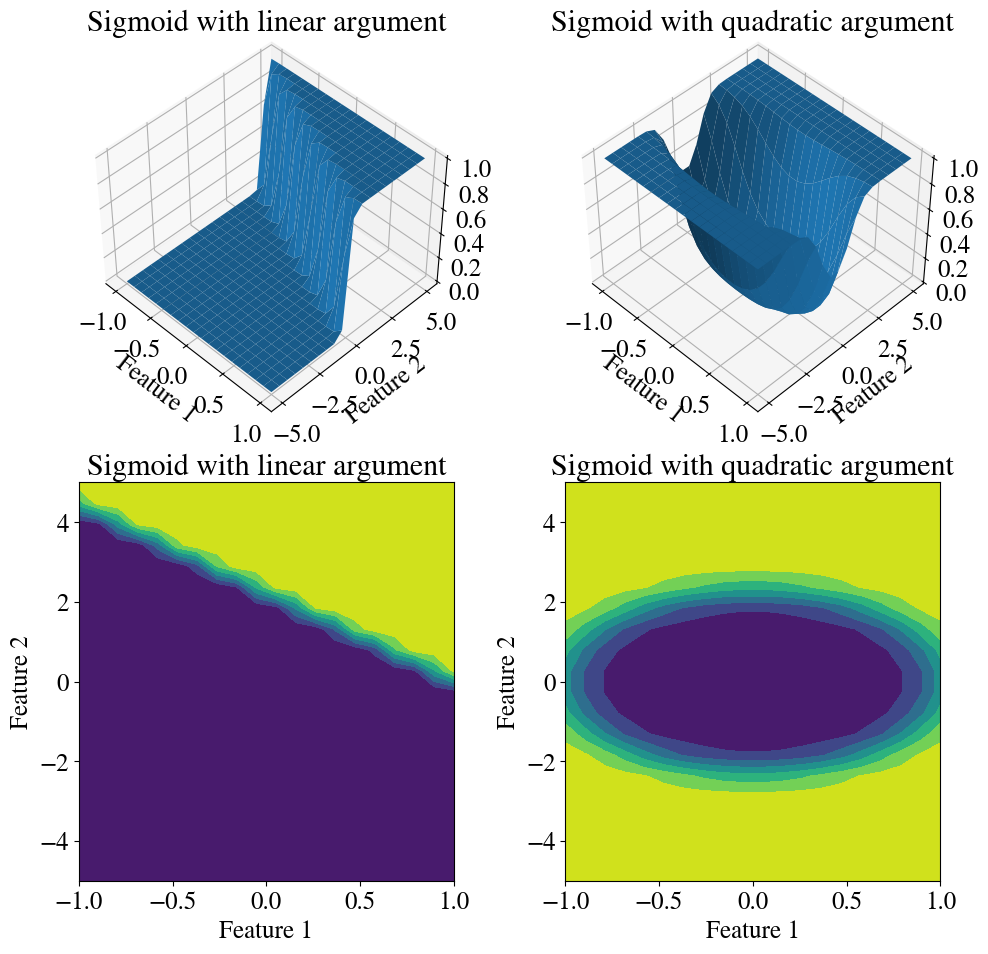
And below are two illustrations of what sigmoid functions can look like when we have additional features, in this case two. In the left panel, \(g(z) = \mathrm{sigmoid}(\mathbf{X}\cdot \vec{\theta})\) for a linear relation \(\mathbf{X}\cdot \vec{\theta} = \theta_0 + \theta_1 x_1 + \theta_2 x_2\). In the right panel, we engineered features that are the squares of each variable, such that we can have \(\mathbf{X}\cdot \vec{\theta} = \theta_0 + \theta_1 x_1^2 + \theta_2 x_2^2\) as the argument of the sigmoid function. For both cases, I consider a constant value of \(\theta_0 = -22\) and vary the fitting parameters \(-1<\theta_1<1\) and \(-5<\theta_2<5\), each with 20 points.

xx = np.linspace(-1,1,20)
yy = np.linspace(-5,5,20)

XX, YY = np.meshgrid(xx,yy)

ZZ = -22 + 22 * XX + 10 * YY

ZZ = sigmoid(ZZ)

# Plotting:
fig = plt.figure(figsize=(10,10))
ax = fig.add_subplot(221, projection='3d')
ax.view_init(45, -45)

plt.title('Sigmoid with linear argument')
ax.plot_surface(XX, YY, ZZ)
plt.xlabel('Feature 1')
plt.ylabel('Feature 2')


ax = fig.add_subplot(223)
plt.title('Sigmoid with linear argument')
ax.contourf(XX, YY, ZZ)
plt.xlabel('Feature 1')
plt.ylabel('Feature 2')

ax = fig.add_subplot(222, projection='3d')
ax.view_init(45, -45)

ZZ = -5 + 5*XX**2 +  YY**2
ZZ = sigmoid(ZZ)

plt.title('Sigmoid with quadratic argument')
ax.plot_surface(XX, YY, ZZ)
plt.xlabel('Feature 1')
plt.ylabel('Feature 2')

ax = fig.add_subplot(224)
plt.title('Sigmoid with quadratic argument')
ax.contourf(XX, YY, ZZ)
plt.xlabel('Feature 1')
plt.ylabel('Feature 2')

plt.tight_layout()

Decision boundary

These is one more important subtlety to discuss regarding the sigmoid function. The sigmoid function is a continuous function, while our target \(y\) is discrete and can only take on the values of 0 or 1. So while the sigmoid hypothesis fits the measurements \(y\) very well in the in the earlier figure above, we can never have any measurements along the steep slopey part between \(0<y<1\). Instead, we can think of the sigmoid hypothesis function as the probability that \(y=1\), as was briefly mentioned above. Given that our machine learning algorithm for binary categorization should only output 0s and 1s (because those are the only values that can be measured), we need to ‘post-process’, if you will, the predictions from the sigmoid function and assign a value of \(\tilde{y}=1\) for all \(h(x,\theta) = g(\mathbf{X}\cdot \vec{\theta})\ge 0.5\) (ommitting vector symbols) and \(\tilde{y}=0\) for all \(h(x,\theta) = g(\mathbf{X}\cdot \vec{\theta})< 0.5\).

Below we define a function that does just that (using some python trickery that you maybe haven’t seen before yet). [As always, if the notation is not clear, create a new code cell and without defining it as a function, run each line inside of it one-by-one to see what it does. ]

def predict(theta,x):
  hypothesis = sigmoid(x.dot(theta))
  p = hypothesis
  p[hypothesis >= 0.5]=1
  p[hypothesis < 0.5]=0
  return p

It is worth (and necessary) digging in a little further. By definition of the sigmoid function, and as illustrated above, \(g(z)\ge 0.5\) for \(z>0\), so \(g(\mathbf{X}\cdot \vec{\theta})\ge0.5\) for \(\mathbf{X}\cdot \vec{\theta}>0\). That means that the decision boundary between malignant and benign tumors (in this particular example) is given by the linear relation \(\mathbf{X}\cdot \vec{\theta} = \theta_0 + \theta_1 x = 0\). Given the best fit \(\theta\) values, \(-22 + 22 x = 0\) (don’t worry yet how I obtained those), we can easily solve this to find: \(x=1\). In other words, a tumor size of \(x=1\) is the precise decision boundary between malign or benign (plotted as a dash-dotted line). The above function will not predict continuous (sigmoid) values, but only values of \(\tilde{y}=1\) for \(x\ge 1\) and \(\tilde{y}=0\) for \(x<1\), which perfectly matches our measurement data for this example.

Hypothesis of logistic regression

Any binary classification scheme can be represented as above. Getting ahead of ourselves a little, the vector notation introduced above also readily generalizes to any number \(n\) of linear or nonlinear (using the same trick as for numerical regression) features.

The hypothesis of logistic regression (i.e. classification schemes) is that the data can be represented not by a multivariate linear model $ = h(x,) = $, but rather

$ = h(x,) = .$

Obviously, this non-linear sigmoid function introduces a bit of extra complexity and non-linearity, but as you will soon see, about 90% of everything you learned about numerical regressions will carry over quite straightforwardly to this seemingly completely different type of problem. We use the exact same notation and definitions of whatever features we want to consider, i.e. a matrix that resembles a spreadsheet with one column of ones for the ‘bias’ feature and then as many columns \(n\) as you’d like to consider for linear and non-linear features of various types. Each feature will be weighted by a fitting parameter \(\theta\), including the bias \(\theta_0\). Just as before, we compute a linear relation \(z = \theta_0 + \theta_1 x_1 + \ldots \theta_n x_n = \mathbf{X}\cdot \vec{\theta}\). The only difference is that we essentially convolve that linear hypothesis with the non-linear sigmoid function as \(\tilde{y}=g(z)\).

The objective of a classification machine learning scheme is therefore also exactly the same as before: find fitting parameters \(\vec{\theta}\) such that the aforementioned hypothesis best fits the measurements. Moreover, you’ll see that we can also use the exact same gradient descent method, and its more advanced alternatives, to find those \(\vec{\theta}\).

Remarkably, the only real difference that we need to discuss is how we define ‘best fit’, which we will do in the following.

Cost function of logistic regression - categorization schemes

Remember that in numerical regression the cost function was defined as the mean-squared-error for \(m\) measurement points labeled by superscript \((i)\) with predictions \(\tilde{y}^{(i)}\) compared to actual measurements \(y^{(i)}\), as: \(J(\vec{\theta}) = \frac{1}{2m} \sum_{i=1}^m ( \tilde{y}^{(i)} - y^{(i)})^2 = \frac{1}{2 m} \sum_{i=1}^m (h(x^{(i)},\theta) - y^{(i)})^2\).

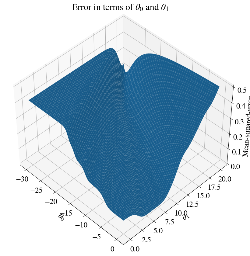
Let’s see what these errors look like when we do a brute-force mapping out of the fitting errors for all combinations of \(-30<\theta_0<0\) and \(0<\theta_1<20\) (with 100 steps in each, for a total of 10,000 combinations of fitting parameters):

nrsteps=100
errors = np.zeros([nrsteps,nrsteps])
theta0 = np.linspace(-30,0,nrsteps)
theta1 = np.linspace(0,20,nrsteps)

for i in range(nrsteps):
  for j in range(nrsteps):
    z = theta0[i] + theta1[j]*x
    hypothesis = sigmoid(z)
    errors[i,j] = mean_squared_error(hypothesis , y)

fig = plt.figure(figsize=(10,10))
ax = fig.add_subplot(111, projection='3d')
ax.view_init(45, -45)

T0, T1 = np.meshgrid(theta0, theta1)

plt.title('Error in terms of '+r'$\theta_0$' + ' and ' +r'$\theta_1$')
ax.plot_surface(T0, T1, errors)

ax.set_xlabel(r'$\theta_0$')
ax.set_ylabel(r'$\theta_1$')
ax.set_zlabel('Mean-squared-error');

You can see that this surface looks far more messy than the ones you saw in the notebook on linear and nonlinear multivariate regressions. The technical/mathematical term for ‘messy’ is that this surface is not convex. If we were to use a gradient descent method based on this error and its slope, you can see it might never converge. Remember that the gradient descent method takes many little steps ‘downhill’ until it finds the minimum of this surface, which is the minimum surface. The analogy to this gradient descent method is that if you put a marble somewhere in this landscape (representing an initial guess for \(\vec{\theta}\)), it should ‘roll down’ to the lowest point. The landscape in the above illustration, though, has many local lowest points (minima). You can see many other local dips that would divert a rolling marble from reaching the absolute minimum. And this is a very simple univariate example.

All of this is because this least-squares error function involves the highly non-linear sigmoid function: \(\mathrm{MSE} (\vec{\theta}) = \frac{1}{m} \sum_{i=1}^m \left(\frac{1}{1+\mathrm{e}^{-\vec{\theta} \vec{x}^{(i)}}} - y^{(i)}\right)^2\), which is messy indeed.

The bottom line is that we need a different measure of how good a given fit is.

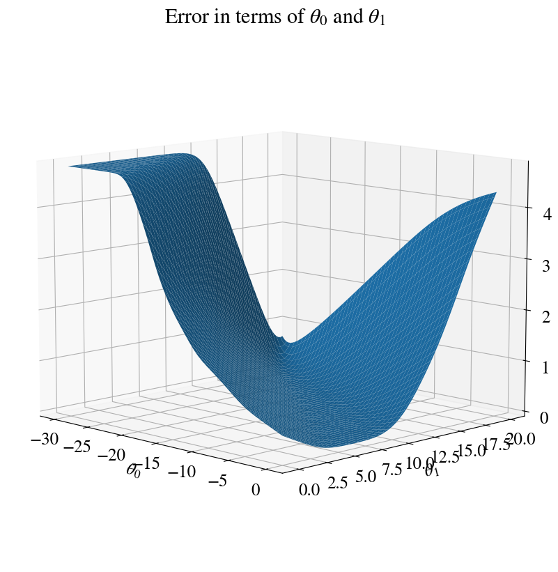
Before even describing how it works, I show below this alternative fitting error (i.e. cost function) over the exact same range in fitting parameters. You see it is much smoother. Indeed, without doing any proof theory here, it has been proven that the cost function introduced next is convex, and has only one minimum. A requirement to use our trusty old gradient descent method.

nrsteps=100
eps = 0.00001
errors = np.zeros([nrsteps,nrsteps])
theta0 = np.linspace(-30,0,nrsteps)
theta1 = np.linspace(0,20,nrsteps)

m = np.size(x)
X = np.append(np.ones([m,1]), x, axis=1)

for i in range(nrsteps):
  for j in range(nrsteps):
    th_vec = np.array([theta0[i],theta1[j]])

    hypothesis = sigmoid(X.dot(th_vec))

    errors[i,j] = - (( np.log(hypothesis+eps).dot(y) +  np.log(1-hypothesis+eps).dot(1-y)) / len(y) ).item()

fig = plt.figure(figsize=(10,10))
ax = fig.add_subplot(111, projection='3d')
ax.view_init(10, -45)

T0, T1 = np.meshgrid(theta0, theta1)

plt.title('Error in terms of '+r'$\theta_0$' + ' and ' +r'$\theta_1$')
ax.plot_surface(T0, T1, errors)

ax.set_xlabel(r'$\theta_0$')
ax.set_ylabel(r'$\theta_1$')
ax.set_zlabel('Error');

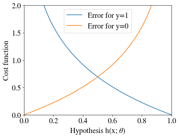
So how do we define our cost function, the measure of how well our hypothesis with a given set of \(\theta\) fits our measured \(y\). For a single measurement point (and therefore omitting those superscripts), and a particular choice of (\(n+1\) length vector) \(\theta\) consider the error:

$J() = { \[\begin{array}{l} -\log(h(x,\theta)) \quad \mbox{if}\quad y=1, \\ -\log(1-h(x,\theta)) \quad \mbox{if}\quad y=0. \end{array}\]

. $

If that doesn’t make intuitive sense, let’s explore this type of error graphically.

xplot = np.linspace(0.001,0.999,50)
plt.xlim(0, 1)
plt.ylim(0, 2)
plt.plot(xplot,-np.log(xplot),label='Error for y=1')
plt.plot(xplot,-np.log(1-xplot),label='Error for y=0')
plt.legend(loc='best');
plt.xlabel('Hypothesis h(x; ' + r'$\theta$' + ')')
plt.ylabel('Cost function');

Remember that the sigmoid hypothesis \(h(x,\theta)\) can only take on \(y\) values between 0 and 1, so that’s the range that is plotted above. Noting the minus sign, \(-\log(h(x,\theta))\) approaches zero when our prediction \(\tilde{y} = h(x,\theta)\) approaches 1. So when the real/measured \(y=1\), the error approaches zero when our hypothesis approaches one, which is what we want. Perhaps more importantly, when the real \(y=1\) but our hypothesis \(\tilde{y} = h(x,\theta)\) is small (approaching the wrong prediction \(\tilde{y}=0\)), the logarithmic function blows up exponentionally (which matplotlib won’t even plot very well). So there is an extremely heavy penalty for a wrong prediction!

When the actual measurement was \(y=0\), the other ‘branch’ of the error function has the exact oposite, and this desired, effect: if the real \(y=0\) but the predicted \(\tilde{y}\) is large (significantly above \(0\)), the error becomes very large, while again the error $-(1-h(x,)) $ approaches zero when indeed \(y=0\).

Rather than having these two ‘branches’ of the error function, which are a bit inelegant and would have some implementation issues, we can combine the two together in a single cost function as follows:

\(J(\theta) = - y \log(h(x,\theta)) -(1-y) \log(1-h(x,\theta)).\)

The reason that this works is, again, because (the real, measured) \(y\) can only take on the values of \(0\) and \(1\). When \(y=1\), the second term is automatically zero and the first term is identical to what we had above (because the extra factor \(y\) is just 1). Similarly, when \(y=0\), the first term vanishes and in the second term \(1-y=1\), such that it is identical to what we had above.

As a minor implementation detail: when we start with an initial guess of all \(\theta =0\) (as we have often done before) the argument of the logarithms is zero and \(\log{0}=\infty\). Just as a safeguard, we add a small constant \(\epsilon\) inside the logarithms to try and avoid infinite values. With that, we code the logistic regression cost function as follows:

def cost_logistic(theta, x, y):
  eps = 0.00001
  hypothesis = sigmoid(x.dot(theta))
  cost = - ( np.log(hypothesis+eps).dot(y) +  np.log(1-hypothesis+eps).dot(1-y)) / len(y)
  return cost

We can also make this a bit fancier with python:

def cost_logistic(theta, x, y, eps=1e-15):
    hypothesis = sigmoid(x.dot(theta))
    hypothesis = np.clip(hypothesis, eps, 1 - eps)
    cost = - (np.log(hypothesis).dot(y) +
              np.log(1 - hypothesis).dot(1 - y)) / len(y)
    return cost

Gradient of cost function

The only remaining component we need for a logistical regression / cartegorization machine learning scheme is the gradient of the cost function, such that we can do gradient descent methods as well as more advanced minimization schemes that also need this gradient. Interestingly and surprisingly, the derivative of the cost function with respect to each \(\theta\), when expressed in terms of the cost function itself, turns out to be exactly the same as for the least-squares error of numerical regression. Schematically: \(\frac{\partial J(\theta)}{\partial \theta} = (g(\mathbf{X}\cdot \vec{\theta}) - \vec{y})\cdot \mathbf{X}\) (where \(\theta\) is the vector of all fitting parameters and \(\mathbf{X}\) is the matrix of all features, including bias, for all measurement points). In other words, the hypothesis is different, but the gradient as expressed in terms of the hypothesis is exactly as before, as you can see in the implementation below:

def grad_logistic(theta,x,y):
  hypothesis = sigmoid(x.dot(theta))
  residual = (hypothesis-y)
  grad = residual.dot(x) / len(y)
  return grad

Of course you can try to derive these derivatives by hand or use a symbolic math software like Mathematica to check this for yourself.

We’ve now coded a complete machine learning algorithm for binary categorization. Let’s try it out. First, initialize our fitting parameters \(\theta\) to zero (or any other initial guess), and augment our measured tumor sizes with a bias feature \(x_0\).

[m,n] = np.shape(x)
thetas = np.zeros(n + 1)
X = np.append(np.ones([m,1]), x, axis=1)

Solve the problem by finding \(\theta\) than minimizes cost function (using accelerated method)

Next, to mix things up a little and show you another powerful python function, we use a different ‘conjugate gradient’ minimization scheme that takes our cost function and its gradient to find the parameters \(\theta\) that result in the lowest cost/error:

fitted_theta = optimize.fmin_cg(cost_logistic, thetas,fprime=grad_logistic, args=(X,Y),gtol=0.001)

Optimization terminated successfully.
         Current function value: 0.001923
         Iterations: 7
         Function evaluations: 27
         Gradient evaluations: 27

You can see how this algorithm too only takes 7 iterations to find a best fit, even though we have a much more nonlinear problem now (due to the sigmoid function).

Below, we plot the results. Also, we use the \(\theta\)s fitted to our learning data to predict whether tumors are benign/malignant for tumor sizes outside of our measurement range. Unlike the high-order polynomial fit above, the sigmoid function with optimized parameters \(\theta\) can exprapolate outside of its training data. The fitting parameters obtained here are actually the ones that I used above to show how a sigmoid function can fit these binary data well.

The last step would be to use the predict function above to turn the continous sigmoid function into only binary 0 and 1 values. That step is not shown in the figure because it perfectly matches the measured \(y\) and cannot be illustrated more clearly.

plt.scatter(x[:7],y[:7],color='blue',marker='o', label='Benign')
plt.scatter(x[7:],y[7:],color='red',marker='x', label='Malignant')

m=100
refined_x = np.ones([m,2])
refined_x[:,1] = np.linspace(-1,5,m)

fit = sigmoid(refined_x.dot(fitted_theta))

plt.plot(refined_x[:,1],fit, color='r')

plt.axhline(y=0.5, color='r', linestyle=':')

plt.xlabel('Tumor size')
plt.ylabel('Benign or Malignant');

Now that we have a functional machine learning algorithm for binary classification of one feature (univariate), let’s try it out on increasingly more complex examples with multiple linear features as well as non-linear features.

Multivariate linear logistic regression

In this next example, we go up one level in complexity and consider multivariate, but still linear, logistic regression. As before, because things are hard to visualize in high-dimensional space, we consider only two independent features. When we code our algorithm in efficient vector notation, as we have above, the number of features can be increased to as many as we want, though, without having to change anything in our code. In fact, the final example uses non-linear polynomial logistical regression where we do ‘feature engineering’ of a number of additional (polynomial) features.

Rather than creating our synthetic data by hand, we import data that are stored somewhere on line.

Load data into pandas dataframe

Pandas has a useful function to read in data from a comma-separated-values file (usually with extension .csv, but here just a .txt textfile), or as below, even from an URL. The data is read into a pandas dataframe data and data.head() shows the first few lines of that data frame so we can see what it looks like.

Note that I stored these data into my own Google Drive. Hopefully there aren’t any authentication issues for you to use these data (let me know!).

sheet_url = 'https://docs.google.com/spreadsheets/d/1X-jEUKsulZIGilE91PxK3Nse968gGW9wDwg0lLxP14c/edit#gid=0'
csv_export_url = sheet_url.replace('/edit#gid=', '/export?format=csv&gid=')
data = pd.read_csv(csv_export_url)

data.head()

	x1	x2	y
0	34.623660	78.024693	0
1	30.286711	43.894998	0
2	35.847409	72.902198	0
3	60.182599	86.308552	1
4	79.032736	75.344376	1

print(f"You can also download the file directly from your browser using link\n {csv_export_url}.\n")

You can also download the file directly from your browser using link
 https://docs.google.com/spreadsheets/d/1X-jEUKsulZIGilE91PxK3Nse968gGW9wDwg0lLxP14c/export?format=csv&gid=0.

We will not actually work with pandas dataframes much in this module and use numpy arrays instead. Below, the .iloc indexing is the only example of some pandas manipulations. Specifically we read the first 2 columns into our features \(x\) and the third column into our target \(y\). In the same line, we then convert the resulting pandas dataframes to numpy arrays, just like the ones we have been working with in the previous modules.

X = data.iloc[:,:2].to_numpy()
Y = data.iloc[:,2].to_numpy()

X_save = X
Y_save = Y

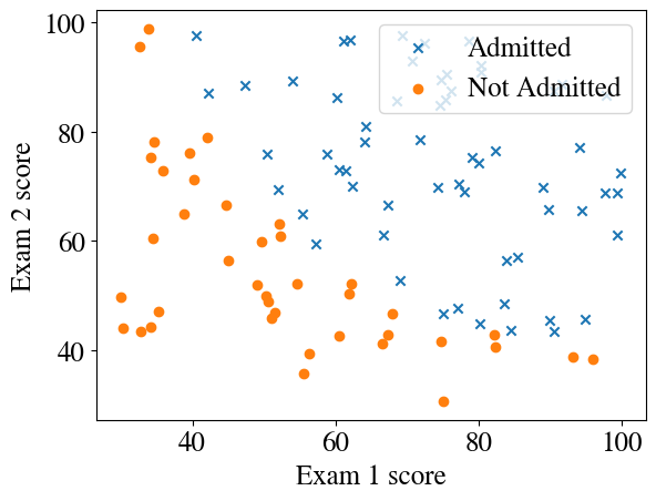
Let’s see what these data look like. The example is from, say, a college admission board which either accepts (\(y=1\)) or rejects (\(y=0\)) student applicants on the combination of two exam scores, say the GRE and GPA to get into graduate school (but scores are converted to percentages). The ‘story’ behind the problem does not really matter; we simply have some binary classification problem, i.e. a yes/no or 1/0 target based on two features \(x_1\) and \(x_2\).

plt.figure()
ax = plt.subplot(111)
pos_ind = np.where(Y==1)
neg_ind = np.where(Y==0)
plt.scatter(X[pos_ind,0], X[pos_ind,1],marker='x')
plt.scatter(X[neg_ind,0], X[neg_ind,1],marker='o')
plt.legend(['Admitted', 'Not Admitted'],loc='upper right')
plt.xlabel('Exam 1 score')
plt.ylabel('Exam 2 score');

Add a column of \(x_0=1\) for the bias feature and define the number of data points \(m\) (training set) and number of features \(n\). Print the first 4 rows of our feature array for inspection.

[m,n] = np.shape(X)
y = Y

x = np.ones([m,n+1])
x[:,1:] = X

print("See what the first 3 lines of X look like:")
x[:4,:]

See what the first 3 lines of X look like:

array([[ 1.       , 34.6236596, 78.0246928],
       [ 1.       , 30.2867108, 43.8949975],
       [ 1.       , 35.8474088, 72.902198 ],
       [ 1.       , 60.1825994, 86.3085521]])

Solve with accelerated minimization scheme

We can solve this Machine Learning problem by using a general-purpose minimization algorithm. All it needs is the (“objective”) function to minimize (the error, or cost function) and its derivatives (cost gradients). We can also specify a tolerance, tol, of what error is acceptable.

initial_theta = np.zeros(n + 1)
Nfeval=1
# The method TNC stands for Truncated Newton Conjugate-Gradient
result = optimize.minimize(cost_logistic, initial_theta, args=(x,y), method='TNC', jac=grad_logistic, \
                           options={'disp': True}, tol=0.00001)


if result.success:
    besttheta = result.x
    nriterations = result.nit
    print("Converged after", result.nit, "iterations to best theta fits:", besttheta)
else:
    print("Accelerated method did not work, maybe try gradient descent.")

Converged after 11 iterations to best theta fits: [-24.70444569   0.2025209    0.19783392]

We will look at the results of this error minimization in more detail in the following sections.

Decision boundary for multivariate linear logistical regression

Below is a somewhat involved function to plot decision boundaries for any number of features, with an easier straight-line option for up to two features, and a more complex option for larger numbers of features. No need to understand this function in detail.

def plotDecisionBoundary(theta, X, y, degree=None, npts=50):
    plt.figure()
    pos_ind = np.where(y == 1)
    neg_ind = np.where(y == 0)
    plt.scatter(X[pos_ind, 1], X[pos_ind, 2], marker='x', label="Class 1")
    plt.scatter(X[neg_ind, 1], X[neg_ind, 2], marker='o', label="Class 0")
    plt.xlabel('Exam 1 score')
    plt.ylabel('Exam 2 score')

    if degree is None or X.shape[1] <= 3:
        # Linear boundary
        plot_x = np.array([X[:, 1].min() - 2, X[:, 1].max() + 2])
        plot_y = -(theta[0] + theta[1]*plot_x) / theta[2]
        plt.plot(plot_x, plot_y, label="Decision boundary")
    else:
        # Nonlinear boundary (polynomial features)
        u = np.linspace(-1, 1.5, npts)
        v = np.linspace(-1, 1.5, npts)
        z = np.zeros((len(u), len(v)))
        for i in range(len(u)):
            for j in range(len(v)):
                feats = generate_polynomials(u[i], v[j], degree)
                z[j, i] = feats.dot(theta)   # note z[j,i] (transpose trick)

        uu, vv = np.meshgrid(u, v)
        plt.contour(uu, vv, z, levels=[0], linewidths=2)

    plt.legend()
    plt.show()

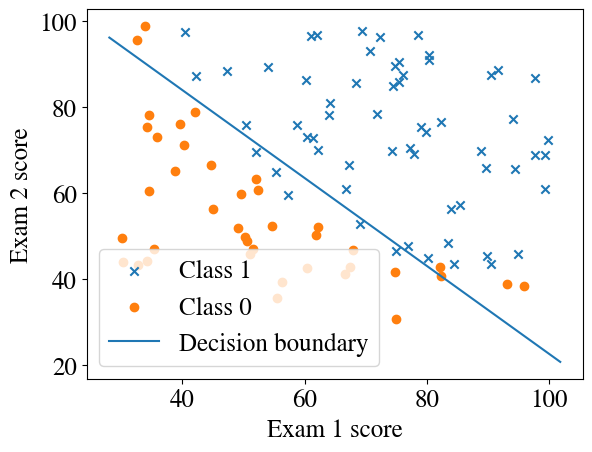
Let’s plot the decision boundary that our algorithm computed.

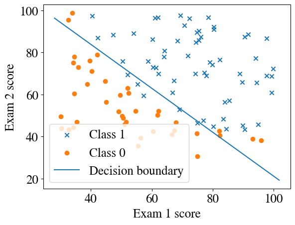
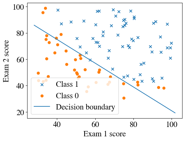
plotDecisionBoundary(besttheta, x, y)

You can see that the straight line, due to our linear combination of the two features (inside the non-linear sigmoid function) separates most, but not all, of the positive and negative binary outcomes. From our predict function, defined above, we can assign 1 to all points above the line and 0 to all points below the decision boundary. Then we can check what fraction of predicted \(\tilde{y}\) are correct (equal to the data \(y\)), as a measure of the success rate of our algorithm.

y_pred = predict(besttheta,x)

print("Accuracy of prediction over entire training set is", np.mean((y_pred == y) * 100), "%")

Accuracy of prediction over entire training set is 89.0 %

Importantly, our best fitting parameters for our hypothesis \(y = h(x,\theta) = g(\mathbf{X}\cdot \theta)\) are given as:

np.round(besttheta,2)

array([-24.7,   0.2,   0.2])

Looking at the figure above, it is clear that there is no straight line that will perfectly separate all the crosses from the circles. We could either use a higher-order nonlinear polynomial logistic regression, which could lead to overfitting, or we can accept that there is noise in our data and this is the most reasonable model, which is probably true in this case.

We will consider another example below, where the separation of our target data \(y\) in terms of features \(x_1\) and \(x_2\) clearly cannot be separated by a straight line and we do indeed need a nonlinear model.

First, though, a demonstration that instead of the ‘black box’ optimization scheme above, it is straightforward to implement the exact same gradient descent method as for numerical regression, but now applied to logistic regression. The only difference in the code below is the form of the cost function, but note that the cost function doesn’t actually even have to be computed at each iteration to update \(\theta\). We only really compute those costs so we can inspect how the cost/error converges and, e.g., plot learning curves.

Gradient descent without black box

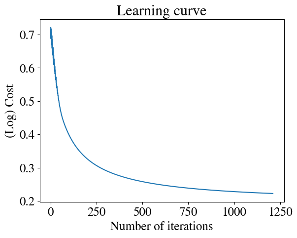
nrsteps = 100000
nr_features = 2

thetas = np.zeros([nrsteps,nr_features+1])
errors = np.zeros(nrsteps)

m = len(y)
alpha = np.array([1,0.001, 0.001]) # note that, after experimentation, I use a much higher learning rate for the intercept than for the other two fitting parameters

# Initial guess:
thetas[0,:] = initial_theta

i=0
converged = False
diverged = False
tolerance = 1e-4

while i < nrsteps-1 and not converged and not diverged:

    errors[i] = cost_logistic(thetas[i,:],x,y)

    thetas[i+1,:] = thetas[i,:] -  alpha * grad_logistic(thetas[i,:],x,y)

    if i>0:
      improvement = np.abs(1- errors[i]/errors[i-1])
      if improvement < tolerance:
        converged = True
        print("Converged in", i, "iterations with error ", round(errors[i],2), "and thetas", np.round(thetas[i,:],2))
      elif improvement > 1:
        print(i, improvement, "Errors are diverging:", errors[i], ">", errors[i-1])
        diverged = True
    i+=1


# Could also add one more safety check:
# if i==nrsteps-1:
#  print(i-1, errors[i-1], errors[i-2],np.abs(1- errors[i-1]/errors[i-2]), "Did not converge in", nrsteps, "steps. Increase nr of steps and try again.")

theta_fit = thetas[i,:]
plt.plot(range(1,i), errors[1:i])
plt.xlabel('Number of iterations')
plt.ylabel('(Log) Cost')
plt.title('Learning curve')


plotDecisionBoundary(theta_fit, x, y)
y_pred = predict(theta_fit,x)
print("Accuracy of prediction over entire training set is", np.mean((y_pred == y) * 100), "%")

Converged in 1210 iterations with error  0.22 and thetas [-15.79   0.13   0.13]

Accuracy of prediction over entire training set is 89.0 %

Not surprisingly, gradient descent finds the same solution, with the same accuracy, as the accelerated scheme used above. From the learning curve, you can see that due to our selection of an appropriate cost/error function (involving those logarithms), the scheme converges smoothly and reasonably fast.

Stochastic Gradient Descent

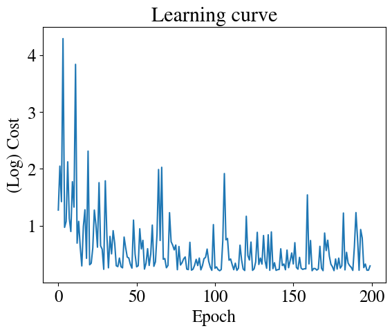
Just for demonstration purposes, we can also use our Stochastic Gradient Descent (SGD) method for logistic regression, just by using the logistic cost function and gradient. As a reminder, SGD work just like gradient descent, except that it fits at one random point at a time instead of all points This makes the learning curve much noisier (see below) but it still converges to a very good solution and at a much lower memory cost.

nr_epochs = 200
nr_features = 2

thetas = []
errors = []

m = len(y)
alpha = np.array([0.1, 0.001, 0.001])   # smaller than batch GD
theta = initial_theta.copy()

for epoch in range(nr_epochs):
    # shuffle data each epoch
    indices = np.random.permutation(m)
    for idx in indices:
        xi = x[idx:idx+1]
        yi = y[idx:idx+1]
        grad = grad_logistic(theta, xi, yi)
        theta -= alpha * grad
    # log error once per epoch
    cost = cost_logistic(theta, x, y)
    errors.append(cost)
    thetas.append(theta.copy())
    if epoch % 10 == 0:
        print(f"Epoch {epoch}, cost {cost:.4f}")

theta_fit = theta

plt.plot(errors)
plt.xlabel('Epoch')
plt.ylabel('(Log) Cost')
plt.title('Learning curve')

plotDecisionBoundary(theta_fit, x, y)
y_pred = predict(theta_fit, x)
print("Accuracy:", np.mean((y_pred == y) * 100), "%")

Epoch 0, cost 1.2755
Epoch 10, cost 1.3276
Epoch 20, cost 0.3126
Epoch 30, cost 1.7906
Epoch 40, cost 0.2794
Epoch 50, cost 0.2766
Epoch 60, cost 1.0113
Epoch 70, cost 0.3010
Epoch 80, cost 0.4165
Epoch 90, cost 0.4304
Epoch 100, cost 0.2503
Epoch 110, cost 0.4144
Epoch 120, cost 1.1667
Epoch 130, cost 0.3247
Epoch 140, cost 0.2271
Epoch 150, cost 0.3272
Epoch 160, cost 0.3273
Epoch 170, cost 0.8716
Epoch 180, cost 0.2537
Epoch 190, cost 1.2314

Accuracy: 91.0 %

The implementation of mini-batch gradient descent is similarly straightforward.

Multivariate and non-linear logistical regression

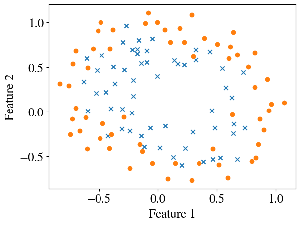
Let’s consider a more complex problem (without specifying what it might be), which can clearly not be resolved by a straight-line decision boundary. In the code below, I download another dataset from my Google Drive into a pandas dataframe, extract features and targets into numpy arrays, and plot the data with matplotlib.

# data = pd.read_csv('http://astro.pas.rochester.edu/~moortgat/ex2data2.txt')
sheet_url = 'https://docs.google.com/spreadsheets/d/1eq-Awuub_ChZi5YIqlbq81_RWUUrFBIqRwVeMZerVUI/edit#gid=0'
csv_export_url = sheet_url.replace('/edit#gid=', '/export?format=csv&gid=')
data = pd.read_csv(csv_export_url)


X = data.iloc[:,:2].to_numpy()
Y = data.iloc[:,2].to_numpy()

plt.figure()
ax = plt.subplot(111)
pos_ind = np.where(Y==1)
neg_ind = np.where(Y==0)
plt.scatter(X[pos_ind,0], X[pos_ind,1],marker='x')
plt.scatter(X[neg_ind,0], X[neg_ind,1],marker='o')
plt.xlabel('Feature 1')
plt.ylabel('Feature 2')

[m,n] = np.shape(X)
y = Y

x = np.ones([m,n+1])
x[:,1:] = X

To separate (categorize) the crosses from the solid circles we clearly need a more complex decision boundary, which basically requires a nonlinear model. So how does this work?

Exactly the same as for numerical regression! To go ‘all in’, below we generate (‘engineer’) additional features up to 6th order, and not just \(x_1^2\), \(x_1^3\), \(\ldots\), \(x_1^6\) (and similar for \(x_2\)), but also every cross-product, such as \(x_1^2 \times x_2^3\) (a 5th order term). In total (including the bias feature) this results in 28 features (!) and we have 117 data points. The dimensions of the feature array are printed below.

X1 = x[:,1]
X2 = x[:,2]
degree = 6;
m = len(X1)
out = np.ones([m,1])
newfeature = np.ones([m,1])

for i in range(1,degree+1):
    for j in range(i+1):
        newfeature[:,0] = (X1**(i-j))*(X2**j)
        out = np.append(out, newfeature, axis=1)
xpoly = out

print("The dimensions of our feature array are now", np.shape(xpoly))

The dimensions of our feature array are now (117, 28)

A more elegant and reusable way to do this would be to define a function to generate these polynomials (remember this function; you may want to use it yourself in current/future labs, perhaps generalized for any number of initial features!):

def generate_polynomials(X1,X2,degree):
  m = np.size(X1)
  out = np.ones([m,1])
  newfeature = np.ones([m,1])

  for i in range(1,degree+1):
      for j in range(i+1):
          newfeature[:,0] = (X1**(i-j))*(X2**j)
          out = np.append(out, newfeature, axis=1)
  return out

Accelerated minimization of cost function

Now we can use the same cost minimization routine to solve this multivariate non-linear logistic regression problem, just like we did above for a simpler problem:

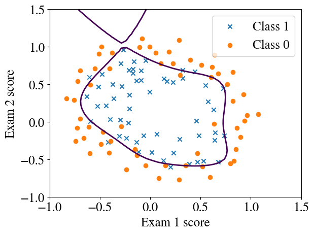
[m,n] = np.shape(xpoly)
initial_theta = np.zeros(n )

result = optimize.minimize(cost_logistic, initial_theta, args=(xpoly,y), method='TNC', jac=grad_logistic, \
                           options={'disp': True}, tol=0.001)

if result.success:
    besttheta = result.x
    nriterations = result.nit
    print("Converged after", result.nit, "iterations to best theta fits:", besttheta)
else:
    print("Accelerated method did not work, maybe try gradient descent.")


y_pred = predict(besttheta,xpoly)
print("Accuracy of prediction over entire training set is", np.mean((y_pred == y) * 100), "%")

Converged after 8 iterations to best theta fits: [  3.34591937   0.64053159   5.23656287  -4.57609633  -9.97955929
   2.15367467   5.68161782   9.09473606  11.55833427  -7.67227824
   1.24670857   3.74354104 -10.97600859   2.23912599 -24.53333639
  -5.08776892  -7.15468391  22.19795878 -10.99513726 -21.84276866
  17.46424809 -19.74693719  -9.53567875  -1.73629378  17.51058997
 -22.53126912 -13.69498793  -0.50133717]
Accuracy of prediction over entire training set is 87.17948717948718 %

Note that the number of steps required to converge to the optimal fit (8) is even less than the number of features (28).

Visualize accelerated minimization results:

finaltheta = besttheta

# Plot the decision boundary and data in one call
plotDecisionBoundary(finaltheta, xpoly, y, degree=degree)

# Accuracy check
y_pred = predict(finaltheta, xpoly)

print("Accuracy of prediction over entire training set is",
      np.round(np.mean((y_pred == y) * 100), 0), "%")

Accuracy of prediction over entire training set is 87.0 %

This example demonstrates how we can compute very complex decision boundaries for binary classification.

Gradient descent

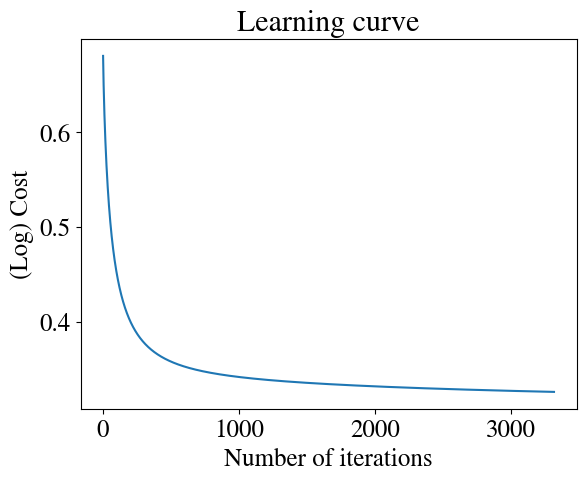
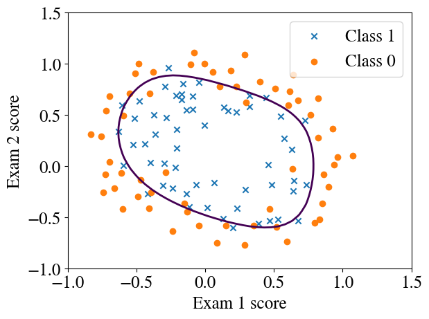
Even this complex problem can also be readily (but less computationally efficiently) be handled by our trusty gradient descent method (i.e. without any external functions). Let’s see how to code this, which you can also use in the lab. You should see that this code is essentially exactly the same as for numerical regression, expect that is uses a different cost function and its gradient.

nrsteps = 100000

thetas = np.zeros([nrsteps,n])
errors = np.zeros(nrsteps)

m = len(y)
alpha = 1

i=0
converged = False
diverged = False
tolerance = 1e-5
while i < nrsteps-1 and not converged and not diverged:

    errors[i] = cost_logistic(thetas[i,:],xpoly,y)
    thetas[i+1,:] = thetas[i,:] -  alpha * grad_logistic(thetas[i,:],xpoly,y)

    if i>10:
      improvement = np.abs(1- errors[i]/errors[i-1])
      if improvement < tolerance:
        converged = True
        print("Converged in", i, "iterations with error ", round(errors[i],2), "and thetas", np.round(thetas[i,:],2))
      elif improvement > 1:
        print(i, improvement, "Errors are diverging:", errors[i], ">", errors[i-1])
        diverged = True
    i+=1


if i==nrsteps-1:
  print(i-1, errors[i-1], errors[i-2],np.abs(1- errors[i-1]/errors[i-2]), "Did not converge in", nrsteps, "steps. Increase nr of steps and try again.")

Converged in 3318 iterations with error  0.33 and thetas [ 3.89  2.55  4.43 -5.3  -5.91 -7.1   1.57 -1.29  0.49 -1.35 -4.92  1.93
 -3.02 -2.41 -4.24 -1.2  -0.53  2.24 -2.44 -2.42  1.14 -4.67  1.15 -1.14
  1.27 -2.38 -2.36 -0.3 ]

Plot the learning curve and decision boundary:

theta_fit = thetas[i,:]

# Learning curve
plt.plot(range(1, i), errors[1:i])
plt.xlabel('Number of iterations')
plt.ylabel('(Log) Cost')
plt.title('Learning curve')

# Prediction + decision boundary
finaltheta = theta_fit
plotDecisionBoundary(finaltheta, xpoly, y, degree=degree)

# Accuracy check
y_pred = predict(finaltheta, xpoly)
print("Accuracy of prediction over entire training set is",
      np.round(np.mean((y_pred == y) * 100), 0), "%")

Accuracy of prediction over entire training set is 85.0 %

The accuracy of this fitted model is slightly lower, but the decision boundary is more reasonable, with the previous one from the accelerated method clearly over-fitted. How to automatically prevent overfitting (called ‘regularization’) will be discussed in a later lecture. You will also learn how this binary categorization scheme can be easily extended to any number of categories using the so-called ‘one-versus-all’ method.

Conclusions

At this point we have covered linear and nonlinear, univariate and multivariate, numerical and logistical regressions. Together, those cover quite a wide range of machine learning applications. Other more complex machine learning algorithms, such as (deep/shallow) neural networks, support vector machines, decision trees, are all just variations of the same concepts, sometimes for efficiency reasons and sometimes to allow for even more nonlinear relations.

For example, as I hope to discuss in a later module, support vector machines use almost exactly the same approach as in this notebook, but the sigmoid function is approximated by straight line segments, which results in some desirable features. Deep neural networks, simply put, compute our same hypothesis, the sigmoid \(g(z) = g(\theta x)\) (omitting vector symbols) for different sets of \(\theta\), and then form linear combinations of those sigmoid hypotheses (just once in a shallow neural network, or several times in a ‘deep’ neural network). This results in highly nonlinear functions of the input features that can fit almost anything, but have the disadvantage that the final results are much harder to interpret (in contrast to the above, where we end up with an actual equation for the decision boundary: a polynomial expression with known/fitted coefficients).

Lab: I personally think the lab for this week is quite exciting. Just a few weeks into the semester, you’ll be able to use our from-scratch logistic regression, i.e. without any “black box” routines and just using basic algebra, for actual handwriting recognition (though of course a somewhat idealized problem). Specifically, you’ll use a training data set of images of lots of hand-written numbers and classify each image as an image of a \(0, 1, \ldots, 9\). In a later lab, you’ll use the exact same logistic regression for the even more complex task of image segmentation and classify each pixel in Sentinel-2 satellite imagery as land or water.

Exercise

If you want to practice a little to see how well you understand this week’s lecture materials, i.e. this notebook, start with the data from the first two-feature example above, the data for which were saved in X_save and Y_save and see if you can put together a quadratic model to find a more accurate decision boundary. Use the generate_polynomials function, or the code inside of it, to engineer quadratic polynomial features.

X = X_save
y = Y_save
degree = 2

Modify the cell below to create a feature array xpoly, which has as collumns \(1\), \(x_1\), \(x_2\), \(x_1^2\), \(x_1 x_2\), \(x_2^2\), \(x_1^2 x_2\), etc. (not necessarily in that order). The code is directly available above.

xpoly = X

If you did it right, in the end your feature array should have 100 rows for the 100 datapoints, and 6 columns for the features. Check by running the code below:

np.shape(xpoly)

(100, 2)

Initialize your guesses \(\theta\) to the right size.

[m,n] = np.shape(xpoly)
initial_theta = np.zeros(n )

And now add a cell with the code to actually solve this problem. You can copy on of the accelerated methods above, or use gradient descent, or both. The result should be 6 best-fit values of \(\theta\). Name that vector/array besttheta. The cell below is a place-holder.

besttheta = initial_theta

Once you have computed besttheta , and assuming everything converged etc., you can run the code below, which will plot the data and the decision boundary based on your quadratic features.

finaltheta =  besttheta
# Here is the grid range
npts = 50
u = np.linspace(20, 100, npts);
v = np.linspace(20, 100, npts);

z = np.zeros([len(u), len(v)]);
# Evaluate z = theta*x over the grid
for i in range(npts):
    for j in range(npts):
      coeff = generate_polynomials(u[i],v[j],degree)
      z[j,i] = coeff.dot(finaltheta)

[m,n] = np.shape(xpoly)
plt.figure()
pos_ind = np.where(y==1)
neg_ind = np.where(y==0)
plt.scatter(xpoly[pos_ind,1], xpoly[pos_ind,2],marker='x')
plt.scatter(xpoly[neg_ind,1], xpoly[neg_ind,2],marker='o')


[uu,vv] = np.meshgrid(u,v)
plt.contour(u,v,z,levels=[0])


y_pred = predict(finaltheta,xpoly)
print("Accuracy of prediction over entire training set is", np.mean((y_pred == y) * 100), "%")

---------------------------------------------------------------------------
ValueError                                Traceback (most recent call last)
/tmp/ipython-input-3569305645.py in <cell line: 0>()
     10     for j in range(npts):
     11       coeff = generate_polynomials(u[i],v[j],degree)
---> 12       z[j,i] = coeff.dot(finaltheta)
     13 
     14 [m,n] = np.shape(xpoly)

ValueError: shapes (1,6) and (2,) not aligned: 6 (dim 1) != 2 (dim 0)

---

✏️ Next up: Practice: Logistic Regression

📖 Next module: Module 5: Data Preprocessing & Pipelines