📖 Review the Lecture notes

🏡 Lab: Predicting House Prices with Linear Regression

In this lab, we’ll apply what we’ve learned about linear regression to a real dataset:
the Ames Housing dataset, which contains information about nearly 3,000 homes sold in Ames, Iowa.

🎯 Goals

By the end of this lab, you will: - Explore the distribution of house prices and motivate the use of log-transformed prices. - Learn how to prepare real-world data for modeling: - Handle missing values (imputation). - Convert categorical variables into numbers (one-hot encoding). - Scale features so they are comparable (Min–Max scaling). - Build and train a Linear Regression model to predict home prices. - Evaluate the model using different error metrics ($R^2$, RMSE, MAE, RMSLE). - Visualize predictions vs. actual prices to see where the model works well and where it struggles. - Put everything together into a scikit-learn Pipeline, which combines preprocessing and modeling into a clean workflow.

🧠 Why this lab?

Machine learning is not just about fitting a model — most of the work is in data preparation.
This lab mirrors the workflow used in practice: 1. Explore the data.
2. Clean and preprocess features.
3. Train a model.
4. Evaluate and visualize performance.
5. Wrap it up in a reusable pipeline.

🗺️ Lab Roadmap

EDA 🔍 → Preprocessing 🛠 → Modeling 📈 → Evaluation 📊 → Pipeline 🧩

👉 By the end, you’ll see how a simple linear model, combined with careful preprocessing, can already achieve strong performance on a challenging real-world dataset.

These are the python packages you will need in this lab.

Code

# Core
import numpy as np
import pandas as pd

# Viz
import matplotlib.pyplot as plt
import seaborn as sns

# Utilities
from pathlib import Path
import joblib  # optional; keep if you plan to save models/pipelines
import gdown   # optional; keep if you download from Google Drive

# Scikit-learn: data prep & modeling
from sklearn.model_selection import train_test_split, KFold
from sklearn.preprocessing import OneHotEncoder, MinMaxScaler  # OneHotEncoder used in demo; MinMax for scaling
from sklearn.impute import SimpleImputer
from sklearn.linear_model import LinearRegression, Ridge, Lasso
from sklearn.metrics import r2_score, mean_squared_error, mean_absolute_error

# Display / style
pd.set_option("display.max_columns", 200)
sns.set_context("talk")

Regression Metrics Overview

When we evaluate regression models, we often look at several metrics together since each emphasizes different aspects of model quality.
Below are the four metrics we’ll report in this lab. Each metric compares predicted target values $\hat{y}$ to ‘ground-truth’ actual/measured values $y$ (the ‘labels’ in our supervised learning models).

1. Coefficient of Determination ($R^2$)

\[ R^2 = 1 - \frac{\sum_i (y_i - \hat{y}_i)^2}{\sum_i (y_i - \bar{y})^2} \]

Interpretation: Proportion of variance in the target $y$ explained by the model.
Range:
- $1.0$: perfect predictions
- $0.0$: no better than always predicting the mean
- Negative: worse than predicting the mean
Units: Unitless (percentage-like, can be multiplied by 100%).
Downside: Can look “good” even when absolute errors are large, especially if the target has high variance.

2. Root Mean Squared Error (RMSE)

\[ \text{RMSE} = \sqrt{\frac{1}{n}\sum_i (y_i - \hat{y}_i)^2} \]

Interpretation: Typical size of the prediction error. Large errors are penalized more because of the square.
Range: $[0, \infty)$ (0 means perfect fit).
Units: Same as the target variable (e.g., dollars for house prices).
Downside: Sensitive to outliers.

3. Mean Absolute Error (MAE)

\[ \text{MAE} = \frac{1}{n}\sum_i |y_i - \hat{y}_i| \]

Interpretation: Average absolute deviation between predictions and true values. Easier to interpret than RMSE.
Range: $[0, \infty)$.
Units: Same as the target variable.
Downside: Less sensitive to large errors than RMSE (so it can “hide” big mistakes).

4. Root Mean Squared Logarithmic Error (RMSLE)

\[ \text{RMSLE} = \sqrt{ \frac{1}{n} \sum_i \left( \log(1+\hat{y}_i) - \log(1+y_i) \right)^2 } \]

Interpretation: Measures relative error on a log scale. Predicting 2× too high is penalized about the same as predicting 2× too low.
Range: $[0, \infty)$.
Units: Unitless (because of the log transform).
Typical scale:
- < 0.2 = excellent (errors ~20% or less on a relative scale)
- 0.2–0.5 = moderate
- 0.5 = large relative errors
Constraint: Only defined for non-negative predictions and targets.

➡️ Best practice: Report all four metrics.
- Use $R^2$ for easy interpretability.
- Use RMSE/MAE for error magnitudes in original units.
- Use RMSLE when relative error matters (e.g., house prices, where \$50k off is minor for a \$1M home but huge for a \$100k home).

I’ll give you a function that computes all these different error/accuracy metrics and outputs them in a clear way using a pandas dataframe:

Code

def evaluate_regression(y_true, y_pred):
    """
    Compute R², RMSE, MAE, and RMSLE for regression predictions.
    Prints a formatted table with nicer display.
    """
    y_true = np.asarray(y_true)
    y_pred = np.asarray(y_pred)

    # Core metrics
    r2   = r2_score(y_true, y_pred)
    rmse = np.sqrt(mean_squared_error(y_true, y_pred))
    mae  = mean_absolute_error(y_true, y_pred)

    # RMSLE (handle non-negative values only)
    if np.any(y_true < 0) or np.any(y_pred < 0):
        rmsle = np.nan
    else:
        rmsle = np.sqrt(mean_squared_error(np.log1p(y_true), np.log1p(y_pred)))

    # Build nicely formatted output
    results = pd.DataFrame({
        "Metric": ["R²", "RMSE", "MAE", "RMSLE"],
        "Value": [
            f"{r2:.0%}",       # percentage
            f"${rmse:,.0f}",   # integer dollars
            f"${mae:,.0f}",    # integer dollars
            f"{rmsle:.3f}"     # 3 decimals
        ]
    })

    print(results.to_string(index=False))
    return results

Ames Housing Dataset — Feature Glossary

In this lab, we’ll have another look at the Ames housing data, which is a good dataset to practice ML pre-processing pipelines, because there are a lot of different types of features. The dataset contains 79 explanatory variables describing residential homes in Ames, Iowa (USA), along with the target variable SalePrice.
Below is a guide to the column names. This is a long text cell, but remember you can collapse this section to hide it when convenient.

Identification

Id: Observation identifier (not a predictive feature).

Sale Information

SalePrice: The property’s sale price in dollars (target variable).

General Property Characteristics

MSSubClass: Building class (coded); e.g. 20 = 1-story 1946+, 60 = 2-story 1946+, 120 = 1-story PUD, etc.
MSZoning: General zoning classification (Residential, Commercial, etc.).
LotFrontage: Linear feet of street connected to property.
LotArea: Lot size in square feet.
Street: Type of road access (Grvl = gravel, Pave = paved).
Alley: Type of alley access (Grvl, Pave, NA = none).
LotShape: General shape of property (Reg = regular, IR1/IR2/IR3 = increasingly irregular).
LandContour: Flatness of the property (Lvl, Bnk, HLS, Low).
Utilities: Type of utilities available (AllPub = all public, NoSeWa = no sewage/water, etc.).
LotConfig: Lot configuration (Inside, Corner, CulDSac, FR2, FR3).
LandSlope: Slope of property (Gtl = gentle, Mod = moderate, Sev = severe).
Neighborhood: Physical location within Ames (e.g., CollgCr, OldTown, Edwards).
Condition1: Proximity to main road or railroad (Artery, Feedr, Norm, etc.).
Condition2: Proximity to a second main road or railroad (if applicable).
BldgType: Type of dwelling (1Fam, 2FmCon, Duplx, TwnhsE, TwnhsI).
HouseStyle: Style of dwelling (1Story, 2Story, 1.5Fin, 1.5Unf, etc.).

House Construction & Age

OverallQual: Overall material and finish quality (1 = very poor, 10 = very excellent).
OverallCond: Overall condition rating (1 = very poor, 10 = very excellent).
YearBuilt: Original construction date.
YearRemodAdd: Remodel date (same as YearBuilt if never remodeled).
RoofStyle: Type of roof (Gable, Hip, Gambrel, Mansard, Flat, Shed).
RoofMatl: Roof material (CompShg = composition shingles, Tar&Grv, WdShngl, etc.).
Exterior1st: Exterior covering on house (brick, siding, stucco, etc.).
Exterior2nd: Exterior covering on house (if more than one material).
MasVnrType: Masonry veneer type (BrkFace, Stone, None).
MasVnrArea: Masonry veneer area in square feet.
ExterQual: Exterior quality (Ex = excellent, Gd, TA = typical, Fa, Po).
ExterCond: Exterior condition (same scale).

Foundation & Basement

Foundation: Type of foundation (BrkTil, CBlock, PConc, Slab, Stone, Wood).
BsmtQual: Basement height (Ex, Gd, TA, Fa, Po, NA).
BsmtCond: Basement condition (same scale).
BsmtExposure: Walkout or garden level walls (Gd, Av, Mn, No).
BsmtFinType1: Finished basement rating (GLQ, ALQ, BLQ, Rec, LwQ, Unf).
BsmtFinSF1: Type 1 finished square feet.
BsmtFinType2: If multiple types of finished basement.
BsmtFinSF2: Type 2 finished square feet.
BsmtUnfSF: Unfinished square feet of basement.
TotalBsmtSF: Total square feet of basement area.

Heating, Cooling & Utilities

Heating: Type of heating (GasA, GasW, Grav, Wall, OthW, Floor).
HeatingQC: Heating quality and condition (Ex, Gd, TA, Fa, Po).
CentralAir: Central air conditioning (Y/N).
Electrical: Electrical system (SBrkr, FuseA, FuseF, FuseP, Mix).

Interior Features

1stFlrSF: First floor square feet.
2ndFlrSF: Second floor square feet.
LowQualFinSF: Low quality finished square feet (all floors).
GrLivArea: Above grade (ground) living area square feet.
BsmtFullBath: Basement full bathrooms.
BsmtHalfBath: Basement half bathrooms.
FullBath: Full bathrooms above grade.
HalfBath: Half baths above grade.
BedroomAbvGr: Bedrooms above grade (does not include basement bedrooms).
KitchenAbvGr: Kitchens above grade.
KitchenQual: Kitchen quality (Ex, Gd, TA, Fa, Po).
TotRmsAbvGrd: Total rooms above grade (does not include bathrooms).
Functional: Home functionality (Typ = typical, Min1, Min2, Mod, Maj1, Maj2, Sev, Sal).
Fireplaces: Number of fireplaces.
FireplaceQu: Fireplace quality (Ex, Gd, TA, Fa, Po, NA).

Garage

GarageType: Garage location (2Types, Attchd, Basment, BuiltIn, CarPort, Detchd).
GarageYrBlt: Year garage was built.
GarageFinish: Interior finish of the garage (Fin, RFn, Unf).
GarageCars: Size of garage in car capacity.
GarageArea: Size of garage in square feet.
GarageQual: Garage quality (Ex, Gd, TA, Fa, Po).
GarageCond: Garage condition (same scale).

Miscellaneous Areas

PavedDrive: Paved driveway (Y, P, N).
WoodDeckSF: Wood deck area in square feet.
OpenPorchSF: Open porch area in square feet.
EnclosedPorch: Enclosed porch area in square feet.
3SsnPorch: Three season porch area in square feet.
ScreenPorch: Screen porch area in square feet.
PoolArea: Pool area in square feet.
PoolQC: Pool quality (Ex, Gd, TA, Fa, NA).
Fence: Fence quality (GdPrv, MnPrv, GdWo, MnWw, NA).
MiscFeature: Miscellaneous feature not covered in other categories (Elev, Gar2, Othr, Shed, TenC, NA).
MiscVal: $Value of miscellaneous feature.

Sale Conditions

MoSold: Month Sold (1–12).
YrSold: Year Sold.
SaleType: Type of sale (WD = Warranty Deed, CWD, VWD, New, COD, ConLD, ConLI, ConLw, Con, Oth).
SaleCondition: Condition of sale (Normal, Abnorml, AdjLand, Alloca, Family, Partial).

Load the Ames Housing data

I put the dataset in my own Google Drive and made a share link for anyone. The code below allows you to download the file straight into your Colab / Google Drive environment.

Code

# View/download file directly from: https://drive.google.com/file/d/1St06441v0dv4dGyImDLsF5vyJQbCqRBM/view?usp=share_link
# if you want to inspect in Excel or something. Otherwise, download into your Google Drive / Colab like this:
gdown.download(id="1St06441v0dv4dGyImDLsF5vyJQbCqRBM", output="AmesHousing.csv", quiet=False)

# The AmesHousing.csv is the same data that we used before with:
# file_url = 'http://jse.amstat.org/v19n3/decock/AmesHousing.txt'
# r = requests.get(file_url);
# open('AmesHousing.txt', 'wb').write(r.content);
# but formatted a bit differently

Downloading...
From: https://drive.google.com/uc?id=1St06441v0dv4dGyImDLsF5vyJQbCqRBM
To: /content/AmesHousing.csv
100%|██████████| 964k/964k [00:00<00:00, 114MB/s]

'AmesHousing.csv'

Load into pandas dataframe:

Code

# Load Kaggle version of Ames Housing dataset
df = pd.read_csv("AmesHousing.csv")

# Drop Id column if present
if "Id" in df.columns:
    df = df.drop(columns=["Id"])

Data shape: (2930, 82)
Columns (first 15): ['Order', 'PID', 'MS SubClass', 'MS Zoning', 'Lot Frontage', 'Lot Area', 'Street', 'Alley', 'Lot Shape', 'Land Contour', 'Utilities', 'Lot Config', 'Land Slope', 'Neighborhood', 'Condition 1']

	Order	PID	MS SubClass	MS Zoning	Lot Frontage	Lot Area	Street	Alley	Lot Shape	Land Contour	Utilities	Lot Config	Land Slope	Neighborhood	Condition 1	Condition 2	Bldg Type	House Style	Overall Qual	Overall Cond	Year Built	Year Remod/Add	Roof Style	Roof Matl	Exterior 1st	Exterior 2nd	Mas Vnr Type	Mas Vnr Area	Exter Qual	Exter Cond	Foundation	Bsmt Qual	Bsmt Cond	Bsmt Exposure	BsmtFin Type 1	BsmtFin SF 1	BsmtFin Type 2	BsmtFin SF 2	Bsmt Unf SF	Total Bsmt SF	Heating	Heating QC	Central Air	Electrical	1st Flr SF	2nd Flr SF	Gr Liv Area	Bsmt Full Bath	Full Bath	Half Bath	Bedroom AbvGr	Kitchen AbvGr	Kitchen Qual	TotRms AbvGrd	Functional	Fireplaces	Fireplace Qu	Garage Type	Garage Yr Blt	Garage Finish	Garage Cars	Garage Area	Garage Qual	Garage Cond	Paved Drive	Wood Deck SF	Open Porch SF	Screen Porch	Pool QC	Fence	Misc Feature	Misc Val	Mo Sold	Yr Sold	Sale Type	Sale Condition	SalePrice
0	1	526301100	20	RL	141.0	31770	Pave	NaN	IR1	Lvl	AllPub	Corner	Gtl	NAmes	Norm	Norm	1Fam	1Story	6	5	1960	1960	Hip	CompShg	BrkFace	Plywood	Stone	112.0	TA	TA	CBlock	TA	Gd	Gd	BLQ	639.0	Unf	0.0	441.0	1080.0	GasA	Fa	Y	SBrkr	1656	0	1656	1.0	1	0	3	1	TA	7	Typ	2	Gd	Attchd	1960.0	Fin	2.0	528.0	TA	TA	P	210	62	0	NaN	NaN	NaN	0	5	2010	WD	Normal	215000
1	2	526350040	20	RH	80.0	11622	Pave	NaN	Reg	Lvl	AllPub	Inside	Gtl	NAmes	Feedr	Norm	1Fam	1Story	5	6	1961	1961	Gable	CompShg	VinylSd	VinylSd	NaN	0.0	TA	TA	CBlock	TA	TA	No	Rec	468.0	LwQ	144.0	270.0	882.0	GasA	TA	Y	SBrkr	896	0	896	0.0	1	0	2	1	TA	5	Typ	0	NaN	Attchd	1961.0	Unf	1.0	730.0	TA	TA	Y	140	0	120	NaN	MnPrv	NaN	0	6	2010	WD	Normal	105000
2	3	526351010	20	RL	81.0	14267	Pave	NaN	IR1	Lvl	AllPub	Corner	Gtl	NAmes	Norm	Norm	1Fam	1Story	6	6	1958	1958	Hip	CompShg	Wd Sdng	Wd Sdng	BrkFace	108.0	TA	TA	CBlock	TA	TA	No	ALQ	923.0	Unf	0.0	406.0	1329.0	GasA	TA	Y	SBrkr	1329	0	1329	0.0	1	1	3	1	Gd	6	Typ	0	NaN	Attchd	1958.0	Unf	1.0	312.0	TA	TA	Y	393	36	0	NaN	NaN	Gar2	12500	6	2010	WD	Normal	172000
3	4	526353030	20	RL	93.0	11160	Pave	NaN	Reg	Lvl	AllPub	Corner	Gtl	NAmes	Norm	Norm	1Fam	1Story	7	5	1968	1968	Hip	CompShg	BrkFace	BrkFace	NaN	0.0	Gd	TA	CBlock	TA	TA	No	ALQ	1065.0	Unf	0.0	1045.0	2110.0	GasA	Ex	Y	SBrkr	2110	0	2110	1.0	2	1	3	1	Ex	8	Typ	2	TA	Attchd	1968.0	Fin	2.0	522.0	TA	TA	Y	0	0	0	NaN	NaN	NaN	0	4	2010	WD	Normal	244000
4	5	527105010	60	RL	74.0	13830	Pave	NaN	IR1	Lvl	AllPub	Inside	Gtl	Gilbert	Norm	Norm	1Fam	2Story	5	5	1997	1998	Gable	CompShg	VinylSd	VinylSd	NaN	0.0	TA	TA	PConc	Gd	TA	No	GLQ	791.0	Unf	0.0	137.0	928.0	GasA	Gd	Y	SBrkr	928	701	1629	0.0	2	1	3	1	TA	6	Typ	1	TA	Attchd	1997.0	Fin	2.0	482.0	TA	TA	Y	212	34	0	NaN	MnPrv	NaN	0	3	2010	WD	Normal	189900

❓ Lab Question

Can you print out the first 15 column names of the dataset and show the first few lines of the dataframe?

💡 Hint

Use .columns to access column names, and slice to the first 15.
Use .head() to show the top rows of the dataframe.

Code

# Print column names

# print first few lines of dataframe

# maybe also print shape of entire dataframe

Exploratory Data Analysis (EDA)

Exploratory Data Analysis (EDA) is the process of getting to know your dataset before jumping into modeling.
It helps us understand the structure, quality, and main patterns in the data.

Goals of EDA

Understand the dataset
- What features (columns) do we have?
- What does the target variable (here: SalePrice) look like?
Summarize
- Basic statistics: min, max, mean, median, standard deviation.
- Frequency counts for categorical features.
Visualize
- Histograms and boxplots to see distributions.
- Scatterplots to check relationships between variables.
- Correlation heatmaps to spot strongly related features.
Detect issues
- Missing values (NaN).
- Outliers or extreme values.
- Features that may need transformation (e.g., skewed data).
Form hypotheses
- Which features might be good predictors?
- Do we expect linear or nonlinear relationships?
- Are some features redundant or overlapping?

In this lab (Ames Housing example)

We’ll start by looking at the target (SalePrice).
Then check numerical features (e.g., living area, lot size, year built).
Explore categorical features (e.g., neighborhood, building type).
Identify missing data that we’ll need to handle later.
Finally, we’ll combine all preprocessing into a single scikit-learn Pipeline.

🧭 Think of EDA as map-making before the journey:
we don’t build a model yet, but we draw the map of the data landscape so we know where to go.

Explore distribution of target values: sale prices

We already did this in the previous lab, but let’s visualize the distribution of sale prices again. First, we define our usual target variable $y$. I’m giving you the code y = df['SalePrice'].copy() to remind you of something important. If you just use y = df['SalePrice'], then $y$ is just a reference, or ‘view’ is the technical term, of df['SalePrice']. What that means is that when you add some value of $y$, rescale all of $y$, etc, then it also changes the same values in df['SalePrice'], which is generally not what you want (not entire safe). So instead we make a .copy() such that the elements of $y$ are now independent of df['SalePrice'].

Code

# Define our target variable y from the SalePrice column in the Ames dataframe:
y = df['SalePrice'].copy()

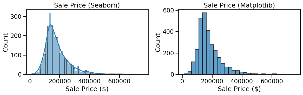
Next, let’s plot the distribution of sales prices as a histogram. I’m showing here how to use the python seaborn library (loaded in the top as sns, similar to plt for matplotlib), which sometimes makes nicer plots than matplotlib. Actually, let’s plot both side-by-side so you can decide which you like better.

Code

fig, axes = plt.subplots(1, 2, figsize=(12,4))

# --- Seaborn version (left) ---
sns.histplot(y, kde=True, ax=axes[0])
axes[0].set_title("Sale Price (Seaborn)")
axes[0].set_xlabel("Sale Price ($)")
axes[0].set_ylabel("Count")

# --- Pure Matplotlib version (right) ---
axes[1].hist(y, bins=30, edgecolor="black", alpha=0.7)
axes[1].set_title("Sale Price (Matplotlib)")
axes[1].set_xlabel("Sale Price ($)")
axes[1].set_ylabel("Count")

plt.tight_layout()
plt.show()

Exploring the Target Variable

❓ Question for you:
Take a look at the histogram of Sale Price.
What does the distribution look like? Is it symmetric, or skewed?

✅ Click here to reveal the answer

The distribution is right-skewed, with a long tail of very expensive houses.

Why does this matter?

Many regression models (especially linear regression) assume that the residuals (errors) are normally distributed and have constant variance (homoscedasticity).
- If the target variable itself is strongly skewed, these assumptions are often violated.
- The model may fit poorly, and errors will be larger for houses at the high end of the price range.

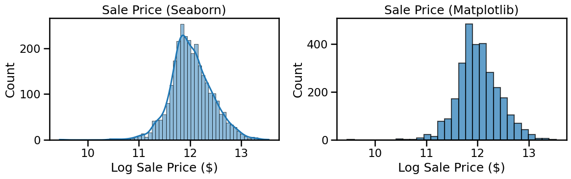
A common solution

Instead of predicting Sale Price directly, we often predict its logarithm:

\[ y' = \log(1 + y) \] if there is a risk of $y$ being zero (avoiding $\log(0)$. In this case, the lowest house price is \$35k so we can just use$$ y’ = (y) $$ - This compresses the long tail.
- The distribution of $ () $ becomes closer to symmetric and bell-shaped.
- Errors are interpreted on a relative scale (percentage differences), which makes more sense for house prices (e.g., being \$50k off on a \$100k house is a big deal, but not on a \$1M house).

Note that after we make any house price predictions, of course we can just take the exponent of $\log(y)$ to get actual house prices and plot those.

➡️ Next, we will define a new target variable as log(SalePrice) and compare the histograms before and after transformation.

Code

# Define a more robust target variable.
# new_y = np.someoperation(y)

❓ Visualize again what this new target variable looks like:

Code

# add plots similar to above

Dropping the target from the feature DataFrame

Now that we’ve defined our target variable (y), it is useful/important to drop it from our DataFrame.
This way, df will only contain the feature columns.

Later, once we have ensured that all features are numeric, we can convert df into a NumPy array for use in scikit-learn models.

💡 Hint

You can drop the target column with: df = df.drop(columns=["SalePrice"]) This removes the SalePrice column from the DataFrame while keeping all the other features.

Code

# remove target column from feature array (still pandas datadframe)

One-Hot-Encoding of Categorical (String) Feature Values

How many categorical features are there?

❓ Question for you:
In the Ames dataset, some features are numerical (e.g. square footage, year built) and some are categorical (e.g. neighborhood, roof type).

Can you figure out how many categorical features there are?
Which ones are they?

Hint: In pandas, categorical features usually have the data type object or category.

❓ Lab Question

Can you figure out how many categorical features there are in the dataset,
and also print their names for reference?

💡 Hint

You can use Python’s len() function to count the items in categorical_cols,
and then just print(categorical_cols) to see the full list.

Code

# Identify categorical features

# Print number of categorical features
# categorical_cols = df.select_dtypes(include=["object", "category"]).columns.tolist(

Number of categorical features: 43

Categorical feature names:
['MS Zoning', 'Street', 'Alley', 'Lot Shape', 'Land Contour', 'Utilities', 'Lot Config', 'Land Slope', 'Neighborhood', 'Condition 1', 'Condition 2', 'Bldg Type', 'House Style', 'Roof Style', 'Roof Matl', 'Exterior 1st', 'Exterior 2nd', 'Mas Vnr Type', 'Exter Qual', 'Exter Cond', 'Foundation', 'Bsmt Qual', 'Bsmt Cond', 'Bsmt Exposure', 'BsmtFin Type 1', 'BsmtFin Type 2', 'Heating', 'Heating QC', 'Central Air', 'Electrical', 'Kitchen Qual', 'Functional', 'Fireplace Qu', 'Garage Type', 'Garage Finish', 'Garage Qual', 'Garage Cond', 'Paved Drive', 'Pool QC', 'Fence', 'Misc Feature', 'Sale Type', 'Sale Condition']

✅ Click here to reveal the correct answer that you should get

The Kaggle Ames dataset has 43 categorical features.
Their names are:

[‘MSZoning’, ‘Street’, ‘Alley’, ‘LotShape’, ‘LandContour’, ‘Utilities’, ‘LotConfig’, ‘LandSlope’, ‘Neighborhood’, ‘Condition1’, ‘Condition2’, ‘BldgType’, ‘HouseStyle’, ‘RoofStyle’, ‘RoofMatl’, ‘Exterior1st’, ‘Exterior2nd’, ‘MasVnrType’, ‘ExterQual’, ‘ExterCond’, ‘Foundation’, ‘BsmtQual’, ‘BsmtCond’, ‘BsmtExposure’, ‘BsmtFinType1’, ‘BsmtFinType2’, ‘Heating’, ‘HeatingQC’, ‘CentralAir’, ‘Electrical’, ‘KitchenQual’, ‘Functional’, ‘FireplaceQu’, ‘GarageType’, ‘GarageFinish’, ‘GarageQual’, ‘GarageCond’, ‘PavedDrive’, ‘PoolQC’, ‘Fence’, ‘MiscFeature’, ‘SaleType’, ‘SaleCondition’]

Handling Missing Values (Imputation)

Real-world datasets almost always have missing values (empty cells, NaN).
In the Ames dataset, some examples include: - LotFrontage (many houses don’t list the frontage length), - Alley (most houses don’t have an alley → marked as missing), - GarageYrBlt (missing when there is no garage).

Why are missing values a problem?

Most machine learning algorithms cannot handle NaN values directly.
We need to decide how to deal with them before modeling.

Options for handling missing data

Drop rows or columns
- Simple, but risky: we may throw away valuable data.
- Only makes sense if very few rows/columns are affected.
Imputation (filling in values)
- Numerical features: replace missing values with the mean, median, or a constant.
- Categorical features: replace with the most frequent category, "Missing", or a special label.
- This keeps all the data but introduces some approximation.
Advanced methods
- Use predictive models (e.g. KNN imputer, regression imputer) to estimate missing values.
- Useful when missingness depends on other features.

In this lab

We will start with simple imputation: - Median for numerical features (robust against outliers). - Most frequent category for categorical features.

Later, we’ll integrate this into a scikit-learn Pipeline so that missing values are automatically handled during training and prediction.

Note: we need to do the impute before the one-hot-encoding in the next step, because we want to impute missing values of categorical values like neighborhood before we turn them into numbers. Remember that: in a pre-processing pipeline, we need to fix missing values before any next steps.

Impute step 1

Check how many measurement points / samples we would lose
if we simply removed rows for houses where one or more feature values are missing. Print the number of rows (measurements/houses) where some feature value is missing, print the total number of measurements $m$ that we started with, and print the difference to see how many measurements/rows we would be left with.

💡 Hint

You can count rows with at least one missing value using:

df.isna().any(axis=1).sum() This works by: * df.isna() → True/False mask of missing values, * .any(axis=1) → True if any value is missing in that row, * .sum() → counts how many rows satisfy that condition.

Code

# Count how many rows have at least one missing value

# Print total number of rows/measurements that we started with

# Print how many rows would remain if we removed all rows with missing values

Number of rows with at least one missing value: 2930
Total rows: 2930
Percentage of rows that would be dropped: 100.0%

Shape after dropping missing rows: (np.int64(0), 81)

What would happen if we dropped all rows with missing values?

❓ We found that dropna() would remove all 2930 rows. Does that make sense?

Yes — in the Ames dataset, every single house has at least one missing value.

Why?
Many features are only applicable to some houses, so they are left as NaN when not relevant:

Alley: missing if the house has no alley.
PoolQC: missing if the house has no pool (most do not).
GarageYrBlt: missing if the house has no garage.
FireplaceQu: missing if the house has no fireplace.
Fence, MiscFeature: often missing as well.

So, almost every row has at least one NaN somewhere.

Are some columns entirely empty?

No — but some have very high percentages of missing values (80–95%).
Examples: PoolQC, MiscFeature, Alley, Fence, FireplaceQu.

Takeaway

Dropping rows with any missing values → disastrous (you lose all data).
Dropping columns with extreme missingness → sometimes reasonable, but be careful:
- Missingness can itself be informative (e.g., “no pool” says something about house price).
The better approach is imputation — filling missing values in a systematic way.

Impute Step 2: Which features have the most missing values?

❓ Task for you

Compute the percentage of missing values for each feature,
then sort the results to find the features with the highest missingness.

Hint: Start with df.isna().mean() — this gives you the fraction of missing values per column. Define this into a separate dataframe. Multiply by 100 to turn it into percentages. Show the .head(10) to see the 10 features with the most missing values.

Code

# Compute % missing values per column

# Show the top 10 columns

	0
Pool QC	99.556314
Misc Feature	96.382253
Alley	93.242321
Fence	80.477816
Mas Vnr Type	60.580205
Fireplace Qu	48.532423
Lot Frontage	16.723549
Garage Yr Blt	5.426621
Garage Finish	5.426621
Garage Cond	5.426621

dtype: float64

✅ Click here to reveal the expected result

When checking the percentage of missing values per column, you should find something like this (values may vary slightly depending on the dataset version):

Pool QC 99.556314
Misc Feature 96.382253
Alley 93.242321
Fence 80.477816
Mas Vnr Type 60.580205
Fireplace Qu 48.532423
Lot Frontage 16.723549
Garage Qual 5.426621
Garage Yr Blt 5.426621
Garage Cond 5.426621

Takeaway

The top four features are missing in 80–99% of houses (e.g., most houses have no pool, no miscellaneous feature, no alley, no fence).
Some features (like Mas Vnr Type, Fireplace Qu, Lot Frontage) have moderate missingness.
A few garage-related features are missing in about 5% of houses.

This is why dropping rows with missing values is not an option — instead we need thoughtful imputation or recoding.

We have to pay attention to our data throughout developing this pipeline. If we have a feature where that value is missing in, say, >80% of measurements, a simple impute with, say, the mean of the available values may be quite misleading. For example, you should see in your last result that >99% of houses have no information on “Pool QC”. If you look in the top of the notebook at all the available features, you’ll see that this is a categorical variable for “pool quality”, which of course is only available if a house indeed has a pool; otherwise, it has no value. Similarly, ’Fireplace Qu” is the quality of the fireplace, which only exists if there is a fireplace to begin with.

Structural Missingness: Basements, Garages, Fireplaces, Pools…

Some features in Ames are only present for a subset of houses: - Not every house has a garage, basement, fireplace, pool, alley, or fence.
- In the dataset, these are recorded as NaN when the feature does not exist.

💡 Hint

Inspect these columns first to see which categories exist and how NaN appears.

Here’s some code where you can see the unique values of some of these structural features.

Code

structural_features = [
    "Garage Yr Blt", "Garage Finish", "Garage Qual", "Garage Cond",
    "Bsmt Qual", "Bsmt Cond", "Bsmt Exposure", "BsmtFin Type 1", "BsmtFin Type 2",
    "Fireplace Qu", "Pool QC", "Alley", "Fence", "Misc Feature"
]

for col in structural_features:
    if col in df.columns:
        print(f"{col}: {df[col].unique()[:10]}")
    else:
        print(f"{col} not found in df")

Garage Yr Blt: [1960. 1961. 1958. 1968. 1997. 1998. 2001. 1992. 1995. 1999.]
Garage Finish: ['Fin' 'Unf' 'RFn' nan]
Garage Qual: ['TA' nan 'Fa' 'Gd' 'Ex' 'Po']
Garage Cond: ['TA' nan 'Fa' 'Gd' 'Ex' 'Po']
Bsmt Qual: ['TA' 'Gd' 'Ex' nan 'Fa' 'Po']
Bsmt Cond: ['Gd' 'TA' nan 'Po' 'Fa' 'Ex']
Bsmt Exposure: ['Gd' 'No' 'Mn' 'Av' nan]
BsmtFin Type 1: ['BLQ' 'Rec' 'ALQ' 'GLQ' 'Unf' 'LwQ' nan]
BsmtFin Type 2: ['Unf' 'LwQ' 'BLQ' 'Rec' nan 'GLQ' 'ALQ']
Fireplace Qu: ['Gd' nan 'TA' 'Po' 'Ex' 'Fa']
Pool QC: [nan 'Ex' 'Gd' 'TA' 'Fa']
Alley: [nan 'Pave' 'Grvl']
Fence: [nan 'MnPrv' 'GdPrv' 'GdWo' 'MnWw']
Misc Feature: [nan 'Gar2' 'Shed' 'Othr' 'Elev' 'TenC']

👉 Notice how NaN appears whenever the feature does not exist (e.g., no garage, no pool).
If we impute these with the most frequent category (e.g., "TA" for “Typical Garage”), that would misrepresent the data.
Instead, it would be smarter to create explicit categories like "NoGarage", "NoBasement", "NoFireplace", etc.

✅ Suggested fill values

Garage: "NoGarage"
Basement: "NoBasement"
Fireplace: "NoFireplace"
Pool: "NoPool"
Alley: "NoAlley"
Fence: "NoFence"
Misc Feature: "None"
For the numeric Garage Yr Blt: use 0 (or possibly copy Year Built)

This is not super interesting, so let me suggest some code to show you how to do this:

Code

# Fill structural missingness with explicit categories
df["Garage Finish"] = df["Garage Finish"].fillna("NoGarage")
df["Garage Qual"]   = df["Garage Qual"].fillna("NoGarage")
df["Garage Cond"]   = df["Garage Cond"].fillna("NoGarage")

df["Bsmt Qual"]      = df["Bsmt Qual"].fillna("NoBasement")
df["Bsmt Cond"]      = df["Bsmt Cond"].fillna("NoBasement")
df["Bsmt Exposure"]  = df["Bsmt Exposure"].fillna("NoBasement")
df["BsmtFin Type 1"] = df["BsmtFin Type 1"].fillna("NoBasement")
df["BsmtFin Type 2"] = df["BsmtFin Type 2"].fillna("NoBasement")

df["Fireplace Qu"] = df["Fireplace Qu"].fillna("NoFireplace")
df["Pool QC"]      = df["Pool QC"].fillna("NoPool")
df["Alley"]        = df["Alley"].fillna("NoAlley")
df["Fence"]        = df["Fence"].fillna("NoFence")
df["Misc Feature"] = df["Misc Feature"].fillna("None")

# Clever trick: Fill Garage Yr Blt with Year Built when missing
# if a house has no garage, that is already encoded in a separate feature
df["Garage Yr Blt"] = df["Garage Yr Blt"].fillna(df["Year Built"])

Now that we’ve made these ‘smarter’ impute changes, copy your earlier code and check again what percentage of values is still missing for each feature.

Code

# Compute % missing values per column

# Show the top 10 columns

	0
Mas Vnr Type	60.580205
Lot Frontage	16.723549
Garage Type	5.358362
Mas Vnr Area	0.784983
Bsmt Full Bath	0.068259
Bsmt Half Bath	0.068259
BsmtFin SF 2	0.034130
Bsmt Unf SF	0.034130
Total Bsmt SF	0.034130
Electrical	0.034130

dtype: float64

Impute Step 3: Remove features with too much missing data

You should see that we don’t have too many features left with tons of missing data, but for illustrative purposes we will remove any features with too many missing data points. We could have done this from the start as an easier (but maybe less predictive) approach when we still had many features with lots of missing data.

👉 Go ahead and remove all features that have missing values for more than 10% of houses.

(You can adjust the threshold as you like — but always check which features you are removing, and ask yourself whether they might actually be useful for predicting house prices.)

💡 Hint

Define some threshold variable to your liking (e.g., 0.1) and then you could obtain a list of column names with something like df.columns[df.isna().mean() > threshold].

You can use the pandas syntax:

df.drop(columns=cols_to_drop, inplace=True) where cols_to_drop is a list of column names that exceed your missing-value threshold.

Code

# Set threshold (here: drop features missing in >5% of houses)

# Find features exceeding the threshold

# Print how many features you're dropping and the names of those features

# Print the shape of your feature array before and after dropping those features

Features to drop (2):
['Lot Frontage', 'Mas Vnr Type']

Original shape: (2930, 81)
Reduced shape: (2930, 79)

Impute Step 4: Basic imputation for remaining missing values

After handling structural missingness (like NoGarage, NoPool, etc.), we still have a few features with true missing values.

👉 To keep things simple, we’ll split features into two groups and impute them differently:

Numerical features
- Fill missing values with the median (robust against outliers).
- Example: Lot Frontage → use the median value (or even better, the median by neighborhood).
Categorical features
- Fill missing values with the most frequent category (the mode).
- Example: if most houses have electrical type "SBrkr", fill missing Electrical with "SBrkr".

Why not use the mean for numeric features?

The mean is sensitive to outliers (e.g., one unusually huge lot).
The median gives a more stable central value.

➡️ Later, when we build pipelines, we’ll use scikit-learn’s SimpleImputer to do this automatically.
For now, let’s do a one-off imputation to clean the dataset.

Impute numerical features and double check that no missing values remain. I’ll show you how to do this for the numerical features, and then you can generalize it below for the categorical features.

Code


# Identify numeric columns
num_cols = df.select_dtypes(include=[np.number]).columns

# Imputer for numerical data: use median
num_imputer = SimpleImputer(strategy="median")

# Apply to numeric columns
df[num_cols] = num_imputer.fit_transform(df[num_cols])

print("Numeric imputation done. Any NaNs left in numeric features?")
print(df[num_cols].isna().sum().sum())

Numeric imputation done. Any NaNs left in numeric features?
0

Impute categorical features and double check that no missing values remain:

Code

# Identify categorical columns
cat_cols = df.select_dtypes(exclude=[np.number]).columns

# Imputer for categorical data: use most frequent (mode)
cat_imputer = SimpleImputer(strategy="most_frequent")

# Apply to categorical columns
# generalize what you did for numerical columns above but now for the categorical features

print("Categorical imputation done. Any NaNs left in categorical features?")
# again, generalize from the code above

# Final check: are there any missing values left at all?
# again, copy from above with correct variable names for the categorical variables

Categorical imputation done. Any NaNs left in categorical features?
0
Total missing values remaining in df: 0

One-Hot Encoding of Categorical Features

Most machine learning algorithms (like linear regression) require numerical input.
But many of our features are categorical (e.g. Neighborhood, RoofStyle, SaleCondition).

👉 One-Hot Encoding (OHE) is the standard way to handle this: - Each category value becomes its own binary column (0 or 1). - Example:
Neighborhood = [CollgCr, OldTown, Edwards]
becomes three columns: Neighborhood_CollgCr, Neighborhood_OldTown, Neighborhood_Edwards.

This way, the model can use categorical information without assuming any numeric ordering.

Pandas has its own way to do one-hot-encoding, as in the demo example below:

Code

# Example: look at the "Neighborhood" column
print("Unique neighborhoods:", df["Neighborhood"].nunique())

# One-hot encode just this column
demo_ohe = pd.get_dummies(df["Neighborhood"], prefix="Neighborhood", dtype=int)
print(demo_ohe.dtypes.head())

demo_ohe.head()

Unique neighborhoods: 28
Neighborhood_Blmngtn    int64
Neighborhood_Blueste    int64
Neighborhood_BrDale     int64
Neighborhood_BrkSide    int64
Neighborhood_ClearCr    int64
dtype: object

	Neighborhood_Gilbert	Neighborhood_NAmes
0	0	1
1	0	1
2	0	1
3	0	1
4	1	0

How to inspect what a function does in Colab

When you are not sure what a function does (like pd.get_dummies), there are a few quick ways to get help:

Hover your mouse over the function name in Colab →
A tooltip will appear with the function signature and a short description.
Use a question mark in code (Jupyter/Colab magic):
```python pd.get_dummies?

scikit-learn has its own way to do one-hot-encoding, which uses similar syntax as when fitting regressions etc.

Code

# from sklearn.preprocessing import OneHotEncoder #loaded in the top

# Initialize the encoder
ohe = OneHotEncoder(sparse_output=False, handle_unknown="ignore")

encoded = ohe.fit_transform(df[["Neighborhood"]])

print("Encoded shape:", encoded.shape)
print(ohe.get_feature_names_out(["Neighborhood"]))

Encoded shape: (2930, 28)
['Neighborhood_Blmngtn' 'Neighborhood_Blueste' 'Neighborhood_BrDale'
 'Neighborhood_BrkSide' 'Neighborhood_ClearCr' 'Neighborhood_CollgCr'
 'Neighborhood_Crawfor' 'Neighborhood_Edwards' 'Neighborhood_Gilbert'
 'Neighborhood_Greens' 'Neighborhood_GrnHill' 'Neighborhood_IDOTRR'
 'Neighborhood_Landmrk' 'Neighborhood_MeadowV' 'Neighborhood_Mitchel'
 'Neighborhood_NAmes' 'Neighborhood_NPkVill' 'Neighborhood_NWAmes'
 'Neighborhood_NoRidge' 'Neighborhood_NridgHt' 'Neighborhood_OldTown'
 'Neighborhood_SWISU' 'Neighborhood_Sawyer' 'Neighborhood_SawyerW'
 'Neighborhood_Somerst' 'Neighborhood_StoneBr' 'Neighborhood_Timber'
 'Neighborhood_Veenker']

The pandas approach is perhaps a bit easier, but the scikit-learn option is prefered when we want to combine all the data preprocessing steps into a single pipeline. First, we’ll do the steps one at a time, though, and keep everything in a pandas dataframe (OneHotEncoder outputs a numpy array, which would be more tedious to put back into the pandas dataframe).

One-Hot Encoding All Categorical Features

❓ Can you do the one-hot-encoding for all categorical columns at once using pandas?

Hint: Earlier we defined a variable categorical_cols that holds the names of all categorical features.

💡 Still stuck? Expand for code suggestion

df = pd.get_dummies(df, columns=categorical_cols, drop_first=False, dtype=int)

Code

# One-hot encode all categorical columns directly in df
print("Original shape:", df.shape)

# one-hot-encode all categorical features at once

Original shape: (2930, 81)

Print the shapes of our feature array before and after the one-hot-encoding and pay attention to how many features we’ve added in turning the categorical features into numerical ones with the one-hot-encoding trick.

Code

# print shape of feature array after one-hot-encoding

# Show the first few rows to inspect

After one-hot encoding: (2930, 318)

	Order	PID	MS SubClass	Lot Frontage	Lot Area	Overall Qual	Overall Cond	Year Built	Year Remod/Add	Mas Vnr Area	BsmtFin SF 1	BsmtFin SF 2	Bsmt Unf SF	Total Bsmt SF	1st Flr SF	2nd Flr SF	Gr Liv Area	Bsmt Full Bath	Full Bath	Half Bath	Bedroom AbvGr	Kitchen AbvGr	TotRms AbvGrd	Fireplaces	Garage Yr Blt	Garage Cars	Garage Area	Wood Deck SF	Open Porch SF	Screen Porch	Misc Val	Mo Sold	Yr Sold	MS Zoning_RH	MS Zoning_RL	Street_Pave	Alley_NoAlley	Lot Shape_IR1	Lot Shape_Reg	Land Contour_Lvl	Utilities_AllPub	Lot Config_Corner	Lot Config_Inside	Land Slope_Gtl	Neighborhood_Gilbert	Neighborhood_NAmes	Condition 1_Feedr	Condition 1_Norm	...	BsmtFin Type 2_LwQ	BsmtFin Type 2_Unf	Heating_GasA	Heating QC_Ex	Heating QC_Fa	Heating QC_Gd	Heating QC_TA	Central Air_Y	Electrical_SBrkr	Kitchen Qual_Ex	Kitchen Qual_Gd	Kitchen Qual_TA	Functional_Typ	Fireplace Qu_Gd	Fireplace Qu_NoFireplace	Fireplace Qu_TA	Garage Type_Attchd	Garage Finish_Fin	Garage Finish_Unf	Garage Qual_TA	Garage Cond_TA	Paved Drive_P	Paved Drive_Y	Pool QC_NoPool	Fence_MnPrv	Fence_NoFence	Misc Feature_Gar2	Misc Feature_None	Sale Type_WD	Sale Condition_Normal
0	1.0	526301100.0	20.0	141.0	31770.0	6.0	5.0	1960.0	1960.0	112.0	639.0	0.0	441.0	1080.0	1656.0	0.0	1656.0	1.0	1.0	0.0	3.0	1.0	7.0	2.0	1960.0	2.0	528.0	210.0	62.0	0.0	0.0	5.0	2010.0	0	1	1	1	1	0	1	1	1	0	1	0	1	0	1	...	0	1	1	0	1	0	0	1	1	0	0	1	1	1	0	0	1	1	0	1	1	1	0	1	0	1	0	1	1	1
1	2.0	526350040.0	20.0	80.0	11622.0	5.0	6.0	1961.0	1961.0	0.0	468.0	144.0	270.0	882.0	896.0	0.0	896.0	0.0	1.0	0.0	2.0	1.0	5.0	0.0	1961.0	1.0	730.0	140.0	0.0	120.0	0.0	6.0	2010.0	1	0	1	1	0	1	1	1	0	1	1	0	1	1	0	...	1	0	1	0	0	0	1	1	1	0	0	1	1	0	1	0	1	0	1	1	1	0	1	1	1	0	0	1	1	1
2	3.0	526351010.0	20.0	81.0	14267.0	6.0	6.0	1958.0	1958.0	108.0	923.0	0.0	406.0	1329.0	1329.0	0.0	1329.0	0.0	1.0	1.0	3.0	1.0	6.0	0.0	1958.0	1.0	312.0	393.0	36.0	0.0	12500.0	6.0	2010.0	0	1	1	1	1	0	1	1	1	0	1	0	1	0	1	...	0	1	1	0	0	0	1	1	1	0	1	0	1	0	1	0	1	0	1	1	1	0	1	1	0	1	1	0	1	1
3	4.0	526353030.0	20.0	93.0	11160.0	7.0	5.0	1968.0	1968.0	0.0	1065.0	0.0	1045.0	2110.0	2110.0	0.0	2110.0	1.0	2.0	1.0	3.0	1.0	8.0	2.0	1968.0	2.0	522.0	0.0	0.0	0.0	0.0	4.0	2010.0	0	1	1	1	0	1	1	1	1	0	1	0	1	0	1	...	0	1	1	1	0	0	0	1	1	1	0	0	1	0	0	1	1	1	0	1	1	0	1	1	0	1	0	1	1	1
4	5.0	527105010.0	60.0	74.0	13830.0	5.0	5.0	1997.0	1998.0	0.0	791.0	0.0	137.0	928.0	928.0	701.0	1629.0	0.0	2.0	1.0	3.0	1.0	6.0	1.0	1997.0	2.0	482.0	212.0	34.0	0.0	0.0	3.0	2010.0	0	1	1	1	1	0	1	1	0	1	1	1	0	0	1	...	0	1	1	0	0	1	0	1	1	0	0	1	1	0	0	1	1	1	0	1	1	0	1	1	1	0	0	1	1	1

5 rows × 318 columns

One-hot encoding increases the dimensionality of your dataset. With more features, models can capture more nuanced patterns — but they can also become more complex, need more data, and may overfit.

Feature Engineering: Creating New Features

❓ What new features could you create from this dataset to better predict house prices?

Here are some ideas inspired by top Kaggle approaches:

2. Total square footage

Combine basement and floors:
- TotalSF = TotalBsmtSF + 1stFlrSF + 2ndFlrSF
(This is one of the strongest predictors of Sale Price)

3. Total number of bathrooms

Combine full and half baths, above and below grade:
- TotalBath = FullBath + 0.5*HalfBath + BsmtFullBath + 0.5*BsmtHalfBath
(Having more bathrooms generally raises house value)

➡️ Feature engineering is about adding new meaningful, interpretable features that help the model capture important relationships not directly visible in the raw dataset.

Code

# --- 1. Age-related features ---
df["HouseAge"] = df["Yr Sold"] - df["Year Built"]
df["YearsSinceRemodel"] = df["Yr Sold"] - df["Year Remod/Add"]
df["GarageAge"] = df["Yr Sold"] - df["Garage Yr Blt"]

# --- 2. Total square footage ---
df["TotalSF"] = df["Total Bsmt SF"] + df["1st Flr SF"] + df["2nd Flr SF"]

# --- 3. Total number of bathrooms ---
df["TotalBath"] = (
    df["Full Bath"]
    + 0.5 * df["Half Bath"]
    + df["Bsmt Full Bath"]
    + 0.5 * df["Bsmt Half Bath"]
)

print("New engineered features added:")
print(["HouseAge", "YearsSinceRemodel", "GarageAge", "TotalSF", "TotalBath"])
df[["HouseAge", "YearsSinceRemodel", "GarageAge", "TotalSF", "TotalBath"]].head()

New engineered features added:
['HouseAge', 'YearsSinceRemodel', 'GarageAge', 'TotalSF', 'TotalBath']

	HouseAge	YearsSinceRemodel	GarageAge	TotalSF	TotalBath
0	50.0	50.0	50.0	2736.0	2.0
1	49.0	49.0	49.0	1778.0	1.0
2	52.0	52.0	52.0	2658.0	1.5
3	42.0	42.0	42.0	4220.0	3.5
4	13.0	12.0	13.0	2557.0	2.5

Correlation and House Prices

Before deciding which features to use in our regression model, we should ask:

Which features are actually related to Sale Price?
- If a feature has little or no correlation with the target, it may not be useful.
Which features are highly correlated with each other?
- If two features carry almost the same information, we may only want to keep one.

What is correlation?

Correlation measures how two variables move together.
A correlation of +1 means they move exactly together (perfect positive linear relationship).
A correlation of –1 means they move in exactly opposite directions (perfect negative linear relationship).
A correlation of 0 means there is no linear relationship.

For example:
- If larger houses always sell for higher prices, then GrLivArea and SalePrice will have a high positive correlation.
- If a feature has almost no relationship with price, its correlation will be near 0.

Tools we’ll use

Pandas .corr() → computes correlation values between numeric features.
Seaborn heatmap → visualizes correlation matrices as a color-coded grid.
Bar charts → useful for showing which features are most correlated with the target.

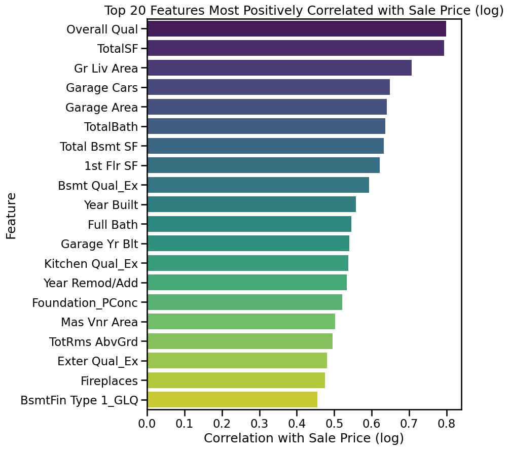
👉 Step 1: Let’s check which features are most correlated with our target SalePrice (we’ll actually use log(SalePrice) since that’s our target).

I’ll give you some code do to this:

Code

# Compute correlations with target (log SalePrice)
corr_with_target = df.corrwith(y).sort_values(ascending=False)

# Top 20 positively correlated features
plt.figure(figsize=(8, 10))
sns.barplot(
    x=corr_with_target.head(20).values,
    y=corr_with_target.head(20).index,
    hue=corr_with_target.head(20).index,   # assign hue explicitly
    dodge=False,
    legend=False,
    palette="viridis"
)
plt.title("Top 20 Features Most Positively Correlated with Sale Price (log)")
plt.xlabel("Correlation with Sale Price (log)")
plt.ylabel("Feature")
plt.show()

❓ Lab Question

We saw the top 20 features most positively correlated with Sale Price.
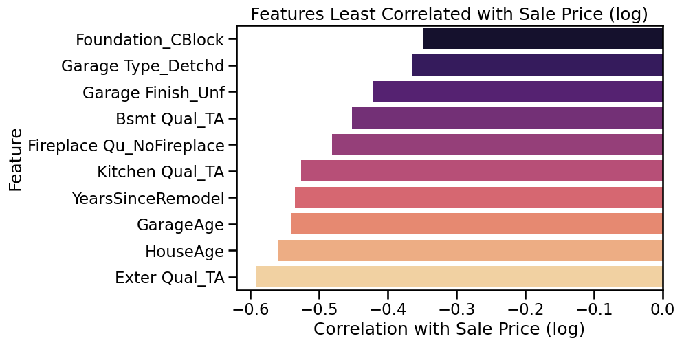
Can you now make a similar plot that shows the least correlated features with Sale Price?

💡 Hint

Instead of using .head(20) on the sorted correlations,
you can use .tail(20) to grab the bottom ones.

Everything else in the plotting code stays almost the same.

Code

# Visualize the 20 features that are least correlated with the known house sales prices, similar to the plots above

Interpreting Correlation

❓ Does correlation assume the relationship between features and Sale Price is linear?

Yes. By default, pandas computes the Pearson correlation, which measures linear relationships:

+1 → perfect positive linear relationship
–1 → perfect negative linear relationship
0 → no linear relationship

What this means:

If a feature has a high correlation with Sale Price, it suggests a strong linear relationship → linear regression can likely use it effectively.
If a feature has low correlation, it might still have a non-linear relationship with Sale Price that Pearson correlation won’t capture.

👉 Correlation is a great first filter for feature selection, but it doesn’t tell the full story.
That’s why we later look at more flexible models (like decision trees or random forests) that can capture non-linear patterns as well.

Feature Selection by Correlation

❓ How can we decide which features to keep based on correlation with Sale Price?

👉 One simple approach is to set a threshold for the absolute correlation:

If |correlation| ≥ 0.1 → keep the feature
If |correlation| < 0.1 → drop the feature

Why?

Features with almost no correlation to the target are unlikely to improve predictions.
Keeping too many noisy or irrelevant features can slow training and sometimes cause overfitting.
This isn’t perfect (correlation only measures linear relationships), but it’s a good first filter.

❓ Lab Question

We don’t need to keep every single feature — some are very weakly correlated with Sale Price.
Let’s filter out features whose correlation with the target is too low.

Can you write code to: 1. Define a correlation threshold (e.g., 0.1).
2. Select only those features where the absolute correlation is above this threshold.
3. Print how many features you kept, and compare it to the original count.
4. Reduce the dataframe df to only these selected features.

(Remember: corr_with_target is already defined, so no need to recompute it!)

💡 Hint

Use abs(corr_with_target) >= threshold to build a mask.
Then grab the feature names with .index.tolist().
Finally, filter df = df[selected_features].

💡 Still stuck? Expand for full code

selected_features = corr_with_target[abs(corr_with_target) >= threshold].index.tolist()

df = df[selected_features]

Add appropriate print statements.

Code

# Set threshold for absolute correlation


# Select features above threshold


# Create reduced DataFrame with only selected features

# Print feature counts before and after dropping features that don't correlate strongly with our target

Selected 152 features (|r| ≥ 0.1):
['PID', 'Lot Frontage', 'Lot Area', 'Overall Qual', 'Overall Cond', 'Year Built', 'Year Remod/Add', 'Mas Vnr Area', 'BsmtFin SF 1', 'Bsmt Unf SF', 'Total Bsmt SF', '1st Flr SF', '2nd Flr SF', 'Gr Liv Area', 'Bsmt Full Bath', 'Full Bath', 'Half Bath', 'Bedroom AbvGr', 'Kitchen AbvGr', 'TotRms AbvGrd', 'Fireplaces', 'Garage Yr Blt', 'Garage Cars', 'Garage Area', 'Wood Deck SF', 'Open Porch SF', 'Enclosed Porch', 'Screen Porch', 'MS Zoning_C (all)', 'MS Zoning_FV', 'MS Zoning_RL', 'MS Zoning_RM', 'Alley_Grvl', 'Alley_NoAlley', 'Lot Shape_IR1', 'Lot Shape_Reg', 'Land Contour_HLS', 'Lot Config_CulDSac', 'Neighborhood_BrkSide', 'Neighborhood_Edwards', 'Neighborhood_IDOTRR', 'Neighborhood_MeadowV', 'Neighborhood_NAmes', 'Neighborhood_NoRidge', 'Neighborhood_NridgHt', 'Neighborhood_OldTown', 'Neighborhood_Sawyer', 'Neighborhood_Somerst', 'Neighborhood_StoneBr', 'Neighborhood_Timber', 'Condition 1_Artery', 'Condition 1_Feedr', 'Condition 1_Norm', 'Condition 2_PosA', 'Bldg Type_1Fam', 'Bldg Type_2fmCon', 'Bldg Type_Duplex', 'Bldg Type_Twnhs', 'House Style_1.5Fin', 'House Style_2Story', 'Roof Style_Gable', 'Roof Style_Hip', 'Roof Matl_WdShngl', 'Exterior 1st_AsbShng', 'Exterior 1st_CemntBd', 'Exterior 1st_HdBoard', 'Exterior 1st_MetalSd', 'Exterior 1st_VinylSd', 'Exterior 1st_Wd Sdng', 'Exterior 2nd_AsbShng', 'Exterior 2nd_CmentBd', 'Exterior 2nd_MetalSd', 'Exterior 2nd_VinylSd', 'Exterior 2nd_Wd Sdng', 'Mas Vnr Type_BrkFace', 'Mas Vnr Type_Stone', 'Exter Qual_Ex', 'Exter Qual_Fa', 'Exter Qual_Gd', 'Exter Qual_TA', 'Exter Cond_Fa', 'Exter Cond_TA', 'Foundation_BrkTil', 'Foundation_CBlock', 'Foundation_PConc', 'Foundation_Slab', 'Bsmt Qual_Ex', 'Bsmt Qual_Fa', 'Bsmt Qual_Gd', 'Bsmt Qual_NoBasement', 'Bsmt Qual_TA', 'Bsmt Cond_Fa', 'Bsmt Cond_NoBasement', 'Bsmt Cond_TA', 'Bsmt Exposure_Av', 'Bsmt Exposure_Gd', 'Bsmt Exposure_No', 'Bsmt Exposure_NoBasement', 'BsmtFin Type 1_BLQ', 'BsmtFin Type 1_GLQ', 'BsmtFin Type 1_NoBasement', 'BsmtFin Type 1_Rec', 'BsmtFin Type 1_Unf', 'BsmtFin Type 2_NoBasement', 'BsmtFin Type 2_Unf', 'Heating QC_Ex', 'Heating QC_Fa', 'Heating QC_Gd', 'Heating QC_TA', 'Central Air_N', 'Central Air_Y', 'Electrical_FuseA', 'Electrical_FuseF', 'Electrical_SBrkr', 'Kitchen Qual_Ex', 'Kitchen Qual_Fa', 'Kitchen Qual_Gd', 'Kitchen Qual_TA', 'Functional_Typ', 'Fireplace Qu_Ex', 'Fireplace Qu_Gd', 'Fireplace Qu_NoFireplace', 'Fireplace Qu_TA', 'Garage Type_Attchd', 'Garage Type_BuiltIn', 'Garage Type_Detchd', 'Garage Finish_Fin', 'Garage Finish_NoGarage', 'Garage Finish_RFn', 'Garage Finish_Unf', 'Garage Qual_Fa', 'Garage Qual_NoGarage', 'Garage Qual_TA', 'Garage Cond_Fa', 'Garage Cond_NoGarage', 'Garage Cond_TA', 'Paved Drive_N', 'Paved Drive_Y', 'Pool QC_Ex', 'Fence_MnPrv', 'Fence_NoFence', 'Sale Type_COD', 'Sale Type_New', 'Sale Type_WD ', 'Sale Condition_Abnorml', 'Sale Condition_Normal', 'Sale Condition_Partial', 'HouseAge', 'YearsSinceRemodel', 'GarageAge', 'TotalSF', 'TotalBath']

Original feature count: 323
Filtered feature count: 152

Next Step: Check for Multicollinearity

❓ We already dropped weakly correlated features — what should we check for now?

We’ve removed features that had little or no correlation with the target.
That’s a good first filter — we no longer carry around lots of noisy features that don’t help predictions.

👉 But we still have to check whether some of the remaining features are highly correlated with each other.

Example: 1st Flr SF, 2nd Flr SF, and TotalSF are all strongly related.
If we keep them all, linear regression may suffer from multicollinearity (unstable coefficients, redundant information).
In such cases, it’s often best to keep only one representative feature.

How to check?

We’ll look at the correlation matrix of all the remaining features and use a heatmap to visualize which ones are strongly correlated with each other.

❓ Lab Question

Now that we’ve filtered down to our most correlated features,
let’s check how strongly they are correlated with each other.

Can you: 1. Compute the correlation matrix of the filtered features, and
2. Plot a heatmap of this matrix?

(Note: you might have called your reduced dataframe df, df_filtered, or something else — use the one you created in the previous step.)

💡 Hint

Use .corr() on your filtered dataframe to compute the correlation matrix.
Then pass this matrix into sns.heatmap() to visualize it.
Don’t forget to set a color map (cmap="coolwarm") and center=0 to highlight positive vs negative correlations.

💡 Still stuck? Expand for full code

# Compute correlation matrix of the filtered features  
corr_matrix = df.corr()   # or df_filtered.corr() depending on your variable name  

# Plot heatmap  
plt.figure(figsize=(14, 12))  
sns.heatmap(  
    corr_matrix,  
    cmap="coolwarm",  
    center=0,  
    square=True,  
    cbar_kws={"shrink": 0.7}  
)  
plt.title("Correlation Heatmap of Selected Features", fontsize=14)  
plt.show()

Code

# Compute correlation matrix of the filtered features

# Plot heatmap ( no grid lines)

Heatmaps with Many Features

With our filtered dataset we still have around 152 features (depending on your choices earlier).
A full correlation heatmap of all these features is very hard to read — the grid looks messy and it’s difficult to spot meaningful patterns.

👉 Instead, we will focus on just the 10 most correlated features with Sale Price.
This will make the heatmap much clearer and serve as an illustrative example of how to check for multicollinearity.

I’ll just give you the code to do this (modify dataframe variable name from df if you changed it earlier):

Code

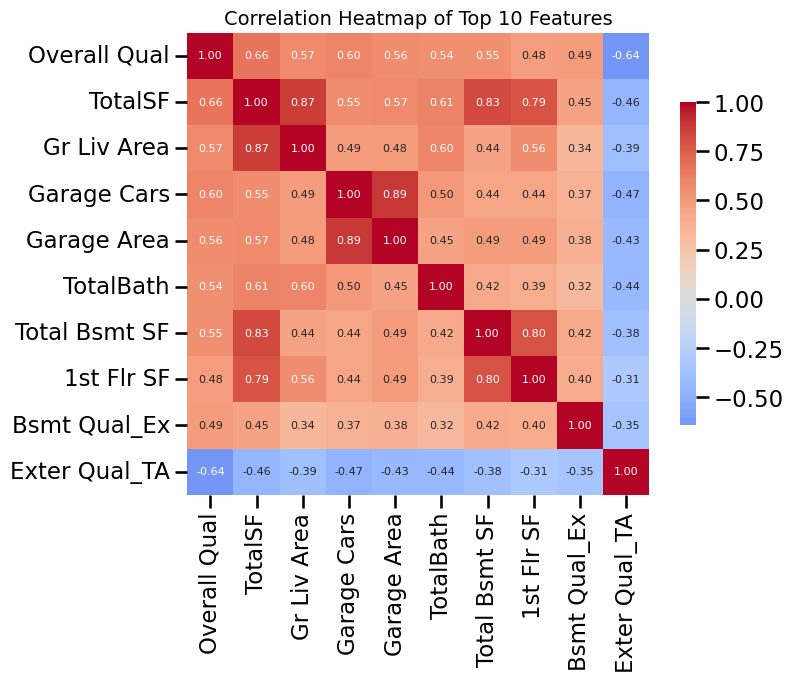
# Find top 10 features most correlated with target
top10_features = df.corrwith(y).abs().sort_values(ascending=False).head(10).index.tolist()

print("Top 10 features most correlated with Sale Price (log):")
print(top10_features)

# Compute correlation matrix for just these features
corr_top10 = df[top10_features].corr()

# Plot heatmap with smaller annotation font
plt.figure(figsize=(8, 6))
sns.heatmap(
    corr_top10,
    annot=True,
    fmt=".2f",
    cmap="coolwarm",
    center=0,
    square=True,
    cbar_kws={"shrink": 0.7},
    annot_kws={"size": 8}   # smaller font size for numbers
)
plt.title("Correlation Heatmap of Top 10 Features", fontsize=14)
plt.show()

Top 10 features most correlated with Sale Price (log):
['Overall Qual', 'TotalSF', 'Gr Liv Area', 'Garage Cars', 'Garage Area', 'TotalBath', 'Total Bsmt SF', '1st Flr SF', 'Bsmt Qual_Ex', 'Exter Qual_TA']

Removing Redundant Features (Multicollinearity)

❓ Some features are strongly correlated with each other — which should we drop?

👉 The common approach is:

Set a correlation threshold (e.g. |r| ≥ 0.8).
For each pair of features that exceed this threshold, keep the one more correlated with the target (SalePrice).
Drop the weaker one.

This reduces multicollinearity and ensures we don’t throw away information that’s predictive of the target.

Note that the correlation matrix, which you should have defined above (for example as corr_matrix) is symmetric, so we only need only the top or bottom triangle. We can do that as follows:

Code

# Select upper triangle of the correlation matrix (ignore self-corr and duplicates)
upper = corr_matrix.where(np.triu(np.ones(corr_matrix.shape), k=1).astype(bool))

Now define some threshold for what features are too correlated to each other can can probably be dropped (maybe 0.8 or so?).

Code

# Set redundancy threshold
# redundancy_threshold =

# Correlation of each feature with the target (log SalePrice)
# use earlier definition of corr_with_target or compute again:
# target_corr = df.corrwith(y).abs()

Number of redundant features to drop: 34
Dropping: ['Exterior 2nd_MetalSd', 'Exterior 2nd_AsbShng', 'Central Air_N', 'Garage Qual_NoGarage', 'Gr Liv Area', 'Electrical_FuseA', 'Kitchen Qual_Gd', 'Exterior 2nd_VinylSd', 'Bsmt Qual_NoBasement', 'Roof Style_Gable', 'Lot Shape_IR1', '1st Flr SF', 'Exterior 2nd_CmentBd', 'Bsmt Cond_NoBasement', 'BsmtFin Type 2_NoBasement'] ...

Remaining feature count: 118

The next step is probably more complicated that I should suggest in this lab, but I can’t help suggest what looks like the best approach: if we have 2 features that are highly correlated, we can drop one of them. But which one? For that, we compare each to how well they correlate to our target variable. In other words, both have similar predictive powers, but we only want to keep the feature with the most predictive power (even if close). Either way, we have to pick one or the other.

So this is what we can do:

🔎 Understanding the Redundancy Removal Code

Here’s the code we used:

to_drop = set()  
for col in upper.columns:  
    high_corr = upper[col][upper[col] > redundancy_threshold].index.tolist()  
    for row in high_corr:  
        # Compare target correlations: drop the weaker one  
        if target_corr[col] >= target_corr[row]:  
            to_drop.add(row)  
        else:  
            to_drop.add(col)

Step by step

upper is the correlation matrix of all features, but only the upper triangle is kept.
This way we only compare each feature pair once (no duplicates).
Outer loop (for col in upper.columns:)
Go through each feature (column) one at a time.
Inner loop (for row in high_corr:)
For this feature (col), find all other features (row) that are highly correlated with it (above our redundancy threshold).
Compare their importance
- Look at how strongly each feature (col and row) correlates with the target (logy).
- If col is more correlated with the target, then we keep col and drop row.
- If row is stronger, then we drop col instead.
Build a drop list
- to_drop is a set of all the weaker features.
- At the end, we drop them all at once from the dataframe.

🔑 Takeaway

Think of it like a pairwise survival game: - Every time two features are “too similar” (highly correlated with each other),
- We only keep the stronger one (the one more correlated with the target).
- The weaker one gets eliminated and added to to_drop.

I’ll just give you the code for this:

Code


# Features to drop (based on lower target correlation in each redundant pair)
to_drop = set()
for col in upper.columns:
    high_corr = upper[col][upper[col] > redundancy_threshold].index.tolist()
    for row in high_corr:
        # Compare target correlations: drop the weaker one
        if target_corr[col] >= target_corr[row]:
            to_drop.add(row)
        else:
            to_drop.add(col)

print(f"Number of redundant features to drop: {len(to_drop)}")
print("Dropping:", list(to_drop)[:15], "...")  # show first 15 for sanity check

# Drop them in place
df = df.drop(columns=list(to_drop))

print("\nRemaining feature count:", df.shape[1])

---------------------------------------------------------------------------
NameError                                 Traceback (most recent call last)
/tmp/ipython-input-3607008411.py in <cell line: 0>()
      1 # Features to drop (based on lower target correlation in each redundant pair)
      2 to_drop = set()
----> 3 for col in upper.columns:
      4     high_corr = upper[col][upper[col] > redundancy_threshold].index.tolist()
      5     for row in high_corr:

NameError: name 'upper' is not defined

Train–Validation Split and Scaling

Before we scale features, we need to split our dataset into training and validation sets.

👉 Why?
- Scaling requires computing the min and max (or mean and std) of each feature.
- If we compute these using the entire dataset, we are “peeking” at the validation data.
- That leaks information from validation into training and gives us overly optimistic results. - I should emphasis that this actually also applies to how we do the imputing, but lets not worry about that for now.

✅ Correct approach:
1. Split into training and validation sets.
2. Fit the scaler on the training set only.
3. Apply the trained scaler to both training and validation sets.

First, convert pandas dataframes to numpy arrays

Code

# Convert features and target to NumPy arrays

# Use whatever variable names you have chosen so far
# X = df.to_numpy()
# logy = logy.to_numpy()

❓ Lab Question

Now it’s time to split our data into two parts: - A training set (used by the model to learn patterns),
- A validation set (used to check how well the model generalizes).

Can you use train_test_split to create: - X_train, X_val (features), and
- y_train, y_val (target values)?

ℹ️ Explanation

test_size=0.2 means that 20% of the data will go into the validation set, and 80% will be used for training.
random_state=42 fixes the random shuffle so you and your classmates all get the same split.
(Any number could be used — 42 is just a convention!)

💡 Hint

from sklearn.model_selection import train_test_split

X_train, X_val, y_train, y_val = train_test_split( X, logy, test_size=0.2, random_state=42 )

👉 Once you have the split, add a print() statement to check the shapes of your training and validation sets.

Code

# Train-validation split (e.g., 80% train, 20% validation)


# Print shapes of training and validation data sets for your inspection

Training set shape: (2344, 118) (2344,)
Validation set shape: (586, 118) (586,)

Scaling and Interpreting Regression Coefficients

When we use Min–Max scaling, each feature is transformed as:

\[ x'_{ij} = \frac{x_{ij} - \text{min}_j}{\text{max}_j - \text{min}_j} \]

where: - $ _j $ = minimum of feature $j$ in the training set
- $ _j $ = maximum of feature $j$ in the training set
- The scaled values $x'_{ij}$ always lie in $[0,1]$.

Why do we care about this?

Linear regression will learn coefficients $ ’_j $ in the scaled feature space.
But those coefficients are hard to interpret, because they apply to normalized units.
To interpret results in the original feature units (square feet, years, number of bathrooms, etc.), we need to “undo” the scaling.

Transforming coefficients back

If we fit a regression in the scaled space:

\[ y = \beta'_0 + \sum_j \beta'_j \, x'_j \]

then the equivalent model in the original feature space is:

\[ y = \beta_0 + \sum_j \beta_j \, x_j \]

with the transformations:

\[ \beta_j = \frac{\beta'_j}{\text{max}_j - \text{min}_j}, \quad \beta_0 = \beta'_0 - \sum_j \frac{\beta'_j \cdot \text{min}_j}{\text{max}_j - \text{min}_j} \]

Takeaway

Fit on scaled features → for stable training.
Transform coefficients back → for human interpretation in original units.

To transform fitting parameters $\beta^\prime$ back into fitting parameters for the original unscaled features $\beta$, we can define a function (though we may not actually use it in this lab):

Code

def unscale_coefficients(beta_scaled, intercept_scaled, scaler):
    """
    Transform regression coefficients and intercept from scaled space
    back to the original feature space.

    Parameters
    ----------
    beta_scaled : array-like, shape (n_features,)
        Coefficients from regression fit on scaled features.
    intercept_scaled : float
        Intercept from regression fit on scaled features.
    scaler : fitted MinMaxScaler
        Scaler used to transform the features.

    Returns
    -------
    beta_orig : np.ndarray, shape (n_features,)
        Coefficients in the original feature space.
    intercept_orig : float
        Intercept in the original feature space.
    """
    scale = scaler.data_max_ - scaler.data_min_
    beta_orig = beta_scaled / scale

    intercept_orig = intercept_scaled - np.sum(beta_scaled * scaler.data_min_ / scale)

    return beta_orig, intercept_orig

Now perform the feature scaling. To emphasize once more: the scaling is based on the min and max of the training data only, and based on those min and max values we also rescale the validation data. So we should not 1) rescale all features based on the min max of the entire dataset (because the validation data are mimicking future measurements) and therefore also not 2) rescale validation data by their own min and max values (because we want this to work for any number of future unseen new measurements).

❓ Lab Question

Next we need to scale our features so they’re all on comparable ranges.
We’ll use Min–Max scaling, which transforms each feature into the range [0, 1].

What to do:

Initialize a MinMaxScaler().
Fit the scaler only on the training data (X_train), and transform it into X_train_scaled.
(We already give you this step in code so you can see the pattern.)
Now, apply the same scaler to the validation data and call the result X_val_scaled.
(Important: never fit on validation data — we only transform it!)
Add some print() statements to check the shapes and display an example of the scaled values.

💡 Hint

Use scaler.transform(X_val) to scale the validation features.
If you’re curious, you can also inspect the scaling factors with:

feature_mins = scaler.data_min_
feature_maxs = scaler.data_max_
feature_scales = scaler.scale_

…but this is not strictly needed for the rest of the lab.

👉 Finally, add two print() statements on your own to check:
- The shapes of the scaled training and validation sets,
- A small sample of scaling values (e.g. the first 5 features).

Code

# Initialize the scaler
scaler = MinMaxScaler()

# Fit only on training data
X_train_scaled = scaler.fit_transform(X_train)

# Apply the same scaling to validation data
# fill this in!


# Print size of scaled training and validation data

# Optionally, add some print statements to check scales and scale factors as you please.

Training set scaled shape: (2344, 118)
Validation set scaled shape: (586, 118)
Example scaling (first 5 features):
Feature 0: min=526301100.00, max=924152030.00, scale=0.0000
Feature 1: min=21.00, max=313.00, scale=0.0034
Feature 2: min=1300.00, max=215245.00, scale=0.0000
Feature 3: min=1.00, max=10.00, scale=0.1111
Feature 4: min=1.00, max=9.00, scale=0.1250

🏡 Time to Train a Model!

We’ve now completed all of our data preprocessing step by step.
The moment has come to actually train a machine learning model and see how well it can predict house prices!

❓ Lab Question

Use a linear regression model to fit the training data and then make predictions on both the training and validation sets.

What to do:

Initialize a regression model.
- The easiest option is LinearRegression from scikit-learn.
- But you are also welcome (and encouraged!) to try your own hand-coded versions of:
  - Gradient Descent
  - Stochastic Gradient Descent
  - Mini-batch Gradient Descent
Fit the model using the scaled training data (X_train_scaled, y_train).
Predict house prices for both the training set and the validation set.

💡 Hint

Here’s the scikit-learn version:

linreg = LinearRegression()
linreg.fit(X_train_scaled, y_train)

y_train_pred = linreg.predict(X_train_scaled)
y_val_pred = linreg.predict(X_val_scaled)

Code

# Initialize and fit linear regression on scaled training data

# Predictions
# make predictions both for the training data and then for the validation data
# save each as something like y_train_pred and y_val_pred
# so we can then compare those predictions to the true values and compute
# accuracy metrics next (below).

Next, we want to compute the accuracy/errors of our predictions versus the ground-truth label values. If you want to see metrics like RMSE or MAE in actual dollar units, though, you have to pay attention to whether or not we modified our target variable early on (e.g. by taking the log of house price instead of just dollar house price). If you did, it makes sense to convert the predicted target values back to just dollars and do the same for the ground truth labels (or just use a separate variable name for those if you still have that defined and didn’t overwrite it with something else).

Code


# Evaluate using our earlier function
print("Training set performance:")

# use the function I provided:  evaluate_regression
# to compute various accuracy metrics between fitted training data and the true values

print("\nValidation set performance:")
# do the same for the validation data

Training set performance:
Metric   Value
    R²     87%
  RMSE $27,868
   MAE $14,321
 RMSLE   0.125

Validation set performance:
Metric   Value
    R²     88%
  RMSE $31,092
   MAE $16,441
 RMSLE   0.124

	Metric	Value
0	R²	88%
1	RMSE	$31,092
2	MAE	$16,441
3	RMSLE	0.124

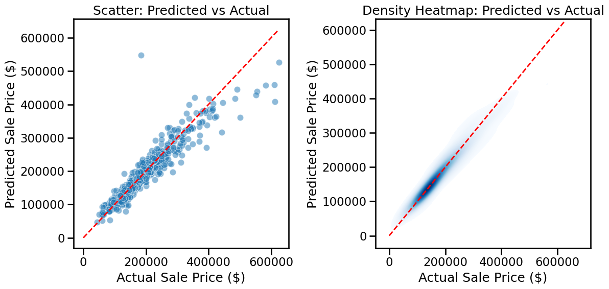
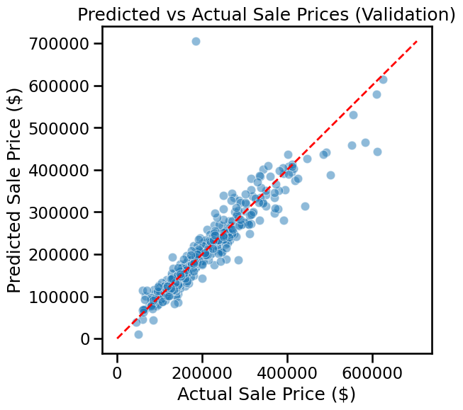
As we did in an earlier lab, it can also be illustrative to plot predicted house prices versus the true sales prices. Doing so as a heat map can give you a sense of the distribution of true/false predictions. In other words, in what price ranges the model is performing better/worse.

Modify the code below as needed for your variable names.

Code

fig, axes = plt.subplots(1, 2, figsize=(12, 6))

# Left: scatter plot
sns.scatterplot(
    x=np.exp(y_val),
    y=np.exp(y_val_pred),
    alpha=0.5,
    ax=axes[0]
)
axes[0].plot(
    [0, np.exp(y_val).max()],
    [0, np.exp(y_val).max()],
    'r--', lw=2
)
axes[0].set_xlabel("Actual Sale Price ($)")
axes[0].set_ylabel("Predicted Sale Price ($)")
axes[0].set_title("Scatter: Predicted vs Actual")

# Right: density heatmap
sns.kdeplot(
    x=np.exp(y_val),
    y=np.exp(y_val_pred),
    fill=True,
    cmap="Blues",
    thresh=0.05,
    levels=100,
    ax=axes[1]
)
axes[1].plot(
    [0, np.exp(y_val).max()],
    [0, np.exp(y_val).max()],
    'r--', lw=2
)
axes[1].set_xlabel("Actual Sale Price ($)")
axes[1].set_ylabel("Predicted Sale Price ($)")
axes[1].set_title("Density Heatmap: Predicted vs Actual")

plt.tight_layout()
plt.show()

Model performance at high prices

❓ Why does the model perform worse for houses above ~$500,000?

Few training examples: Most homes in Ames cost $100k–$250k. Luxury homes are rare, so the model has little data to learn from.
Different drivers of value: Expensive homes often depend on factors not well captured in our dataset (prestige, architecture, location desirability).
Model limitations: A simple linear regression struggles when the relationships between features and prices are not strictly linear.

👉 This means our model tends to underpredict expensive homes because it hasn’t seen enough examples and can’t capture their unique patterns.

⭐ Optional Exercise

Very expensive homes can sometimes distort model performance.
For practice, try removing homes with Sale Prices above $500,000 from both the training and validation sets.

Then:
1. Fit a new Linear Regression model on the filtered data.
2. Evaluate its accuracy again on both training and validation sets.
3. Compare the results to the original model — what changes?

💡 Hint (expand for code)

# Exclude houses above $500,000  
mask_train = np.exp(y_train) <= 500000  
mask_val   = np.exp(y_val) <= 500000  

X_train_sub = X_train_scaled[mask_train]  
y_train_sub = y_train[mask_train]  
X_val_sub   = X_val_scaled[mask_val]  
y_val_sub   = y_val[mask_val]  

print("Filtered training set shape:", X_train_sub.shape, y_train_sub.shape)  
print("Filtered validation set shape:", X_val_sub.shape, y_val_sub.shape)  

# Fit a new linear regression  
linreg_sub = LinearRegression()  
linreg_sub.fit(X_train_sub, y_train_sub)  

# Predictions  
y_train_sub_pred = linreg_sub.predict(X_train_sub)  
y_val_sub_pred   = linreg_sub.predict(X_val_sub)  

# Evaluate performance in $ again  
print("Training set performance (prices <= $500k):")  
evaluate_regression(np.exp(y_train_sub), np.exp(y_train_sub_pred))  

print("\nValidation set performance (prices <= $500k):")  
evaluate_regression(np.exp(y_val_sub), np.exp(y_val_sub_pred))```  

</details>

::: {#_ro1VJ8IyWzU .cell execution_count=3}
``` {.python .cell-code}

# optional. you could try if your model performs better when excluding the most expensive houses.

:::

Reading:

This concludes the part where you are expected to write your own code. Spend the rest of your time reading through the next sections in which:

I give you a primer on Cross-Validation, which we’ll discuss more next week.
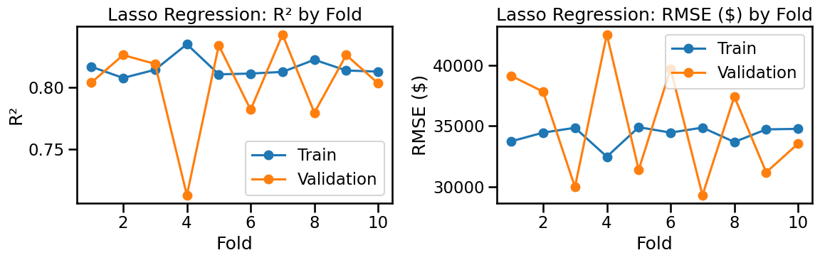
You’ll see some examples of Lasso and Ridge Regularization, which can automatically reduce overfitting (also discussed properly next week).
Importantly in the context of this week’s materials and your work so far in the lab above, you’ll see how we can combine all the pre-processing steps into an elegant and reusable data pre-processing pipeline for machine learning.

Next Steps

In several labs so far, we’ve done a single split of our datasets into training and validation data. Especially for relatively modest sizes of data, which we generally have in this course to make models run fast, the ‘luck of the draw’ is quite a significant factor. In other words, which measurements you pick for training versus validation can have quite a big impact. For example, your training data may not cover the full range of possible values and you should know by know that extrapolating models is often problematic, so if your validation data fall outside the range of your training data you’re often in trouble.

Even when you have more data, though, the best practice is to do so-called cross-validation. This simply means doing a randomized split of your data into training and validation data multiple times. For each split, you fit on the training data and evaluate performance on the validation data. If your model is good (complex enough but not too complex) and you have enough training data, the performance (accuracy) of predictions on un-seen validation data should be the same or similar to the performance on validation data. Also, the performance on both training and validation data should ideally be the same/similar regardless of how you sample the data, i.e. regardless of your random training-validation splits

We’ll discuss this in the next lecture (through this is most of what you need to know), but below I give you some examples of this. There are very easy-to-use built-in functions in scikit-learn, but below I choose to do the cross-validation a bit more explicitly in a loop and use the same pre-processing steps as before.

One critical take-away point that you should burn into your memory is that for each training-validation split, any pre-processing steps can only rely on information from the training data and can never ‘look at’ the validation data, because the validation data are supposed to mimick future measurements that we have not yet taken. So we are not supposed to know what, e.g., the maximum and minimum values of future measurements might me. This is a extremely common mistake by beginner ML users. I’ll keep mentioning this. Never do min-max scaling, imputing, etc on all your data and do a training-validation split afterwards, because by doing so you will have poluted your validation data.

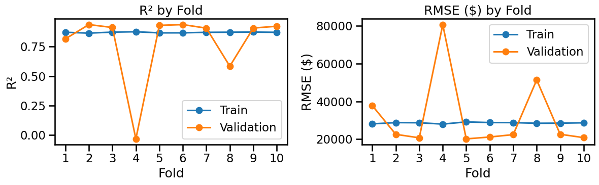
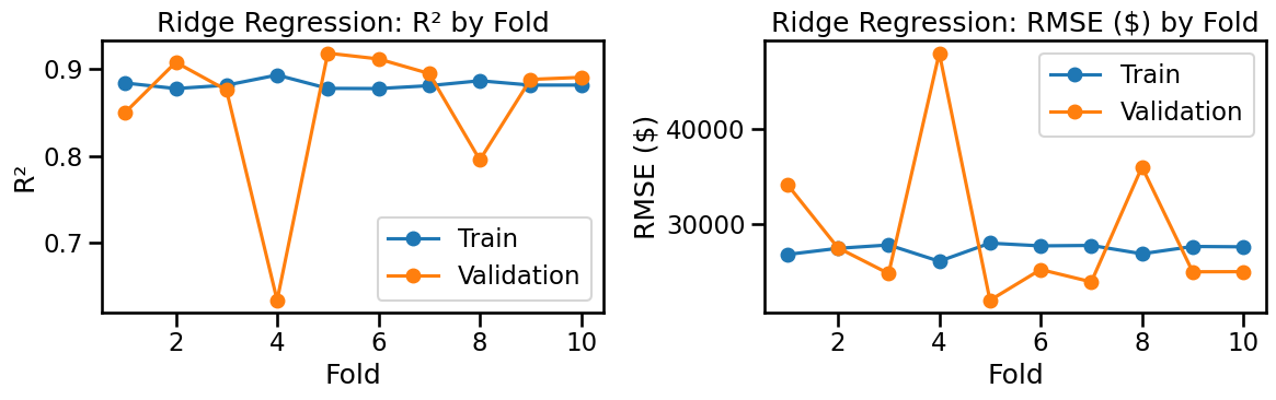
A First Look at Cross-Validation (manual 10-fold)

We’ll do a simple manual 10-fold cross-validation with the exact steps we used before:

Split indices into 10 folds (each fold gets a turn as validation).
For each fold:
- Fit MinMaxScaler on the training split only (no leakage).
- Train a LinearRegression on the scaled training split (target = log price).
- Predict on both training & validation splits (in log space).
- Convert predictions back to dollars with np.exp(...).
- Compute our usual metrics (R², RMSE, MAE, RMSLE) in dollars.
Aggregate the metrics across folds and plot training vs validation to see under/overfitting patterns.

Code

# --- Inputs expected to already exist from your notebook:
# X  -> full numeric feature matrix (np.array), shape (n_samples, n_features)
# logy -> log-transformed target (np.array), shape (n_samples,)

k = 10
kf = KFold(n_splits=k, shuffle=True, random_state=42)

records = []

for fold, (tr_idx, va_idx) in enumerate(kf.split(X), start=1):
    X_tr, X_va = X[tr_idx], X[va_idx]
    y_tr_log, y_va_log = logy[tr_idx], logy[va_idx]

    # Fit scaler on training split only
    scaler = MinMaxScaler()
    X_tr_s = scaler.fit_transform(X_tr)
    X_va_s = scaler.transform(X_va)

    # Fit linear regression
    model = LinearRegression()
    model.fit(X_tr_s, y_tr_log)

    # Predictions in log space
    y_tr_pred_log = model.predict(X_tr_s)
    y_va_pred_log = model.predict(X_va_s)

    # Convert to dollars for human-friendly metrics
    y_tr = np.exp(y_tr_log)
    y_va = np.exp(y_va_log)
    y_tr_pred = np.exp(y_tr_pred_log)
    y_va_pred = np.exp(y_va_pred_log)

    # Metrics (same formulas as evaluate_regression, but numeric for aggregation)
    def metrics(y_true, y_hat):
        r2   = r2_score(y_true, y_hat)
        rmse = np.sqrt(mean_squared_error(y_true, y_hat))
        mae  = mean_absolute_error(y_true, y_hat)
        rmsle = np.sqrt(mean_squared_error(np.log1p(y_true), np.log1p(y_hat)))
        return r2, rmse, mae, rmsle

    r2_tr, rmse_tr, mae_tr, rmsle_tr = metrics(y_tr, y_tr_pred)
    r2_va, rmse_va, mae_va, rmsle_va = metrics(y_va, y_va_pred)

    records.append({
        "fold": fold,
        "R2_train": r2_tr, "RMSE_train": rmse_tr, "MAE_train": mae_tr, "RMSLE_train": rmsle_tr,
        "R2_val":   r2_va, "RMSE_val":   rmse_va, "MAE_val":   mae_va, "RMSLE_val":   rmsle_va
    })

cv_df = pd.DataFrame(records).set_index("fold")
display(cv_df.style.format({
    "R2_train": "{:.3f}", "R2_val": "{:.3f}",
    "RMSE_train": "{:,.0f}", "RMSE_val": "{:,.0f}",
    "MAE_train": "{:,.0f}", "MAE_val": "{:,.0f}",
    "RMSLE_train": "{:.3f}", "RMSLE_val": "{:.3f}",
}))

# Print mean ± std summary
summary = pd.DataFrame({
    "Metric": ["R²", "RMSE ($)", "MAE ($)", "RMSLE"],
    "Train (mean ± std)": [
        f"{cv_df['R2_train'].mean():.3f} ± {cv_df['R2_train'].std():.3f}",
        f"{cv_df['RMSE_train'].mean():,.0f} ± {cv_df['RMSE_train'].std():,.0f}",
        f"{cv_df['MAE_train'].mean():,.0f} ± {cv_df['MAE_train'].std():,.0f}",
        f"{cv_df['RMSLE_train'].mean():.3f} ± {cv_df['RMSLE_train'].std():.3f}",
    ],
    "Val (mean ± std)": [
        f"{cv_df['R2_val'].mean():.3f} ± {cv_df['R2_val'].std():.3f}",
        f"{cv_df['RMSE_val'].mean():,.0f} ± {cv_df['RMSE_val'].std():,.0f}",
        f"{cv_df['MAE_val'].mean():,.0f} ± {cv_df['MAE_val'].std():,.0f}",
        f"{cv_df['RMSLE_val'].mean():.3f} ± {cv_df['RMSLE_val'].std():.3f}",
    ]
})
print("\nCross-Validation Summary (mean ± std across folds):")
print(summary.to_string(index=False))

# --- Plots: Training vs Validation across folds
fig, axes = plt.subplots(1, 2, figsize=(12, 4))

# R²
axes[0].plot(cv_df.index, cv_df["R2_train"], marker="o", label="Train")
axes[0].plot(cv_df.index, cv_df["R2_val"], marker="o", label="Validation")
axes[0].set_title("R² by Fold")
axes[0].set_xlabel("Fold")
axes[0].set_ylabel("R²")
axes[0].set_xticks(cv_df.index)
axes[0].legend()

# RMSE ($)
axes[1].plot(cv_df.index, cv_df["RMSE_train"], marker="o", label="Train")
axes[1].plot(cv_df.index, cv_df["RMSE_val"], marker="o", label="Validation")
axes[1].set_title("RMSE ($) by Fold")
axes[1].set_xlabel("Fold")
axes[1].set_ylabel("RMSE ($)")
axes[1].set_xticks(cv_df.index)
axes[1].legend()

plt.tight_layout()
plt.show()

	R2_train	RMSE_train	MAE_train	RMSLE_train	R2_val	RMSE_val	MAE_val	RMSLE_val
fold
1	0.873	28,115	14,203	0.123	0.817	37,762	17,270	0.135
2	0.866	28,782	14,533	0.126	0.938	22,578	15,166	0.112
3	0.874	28,708	14,627	0.125	0.913	20,734	14,318	0.122
4	0.877	27,993	13,733	0.119	-0.032	80,594	17,380	0.174
5	0.868	29,155	14,628	0.124	0.931	20,171	14,008	0.143
6	0.868	28,797	14,583	0.122	0.938	21,165	13,888	0.147
7	0.872	28,775	14,537	0.126	0.908	22,427	15,073	0.112
8	0.873	28,431	13,893	0.120	0.585	51,334	17,078	0.160
9	0.874	28,491	14,561	0.125	0.909	22,613	15,098	0.119
10	0.872	28,689	14,590	0.125	0.924	20,836	14,001	0.126


Cross-Validation Summary (mean ± std across folds):
  Metric Train (mean ± std) Val (mean ± std)
      R²      0.872 ± 0.004    0.783 ± 0.306
RMSE ($)       28,594 ± 345  32,021 ± 19,849
 MAE ($)       14,389 ± 329   15,328 ± 1,406
   RMSLE      0.123 ± 0.002    0.135 ± 0.021

Why is validation performance more variable than training?

❓ Why do we see much more spread in validation performance than in training performance?

Training scores are stable: Each fold’s training set is ~80% of the data (≈2300 houses). With that much data, the model fits consistently, so training metrics don’t change much.
Validation scores vary more: Each validation set is only ~20% (≈580 houses). Some folds may include more unusual or expensive homes, which are harder to predict. This makes validation performance fluctuate a lot more.
Smaller sample effect: With fewer samples, outliers matter more. One validation fold with a few luxury $500k+ homes can drag performance down, while another fold without them looks much better.

How can we reduce this variation?

Use cross-validation averages: By combining results from multiple folds, we get a more reliable estimate of the model’s true generalization performance.
Collect more data: Larger validation sets reduce sensitivity to outliers.
Apply regularization (Ridge, Lasso): This can reduce overfitting to small quirks in each training set, which should make validation performance more stable.

👉 Next week, when we introduce regularization, we’ll test this idea and see if Ridge/Lasso help reduce variability in validation scores.

Without explaining how Lasso regularization works yet (next week), let me give you a teaser of how it can improve our regression results. We run the exact same code as above, but using the scikit-learn Lasso regression model instead of LinearRegression.

Code

from sklearn.linear_model import Lasso

k = 10
kf = KFold(n_splits=k, shuffle=True, random_state=42)

records_lasso = []

for fold, (tr_idx, va_idx) in enumerate(kf.split(X), start=1):
    X_tr, X_va = X[tr_idx], X[va_idx]
    y_tr_log, y_va_log = logy[tr_idx], logy[va_idx]

    # Fit scaler on training split only
    scaler = MinMaxScaler()
    X_tr_s = scaler.fit_transform(X_tr)
    X_va_s = scaler.transform(X_va)

    # Lasso model
    lasso = Lasso(alpha=0.005, max_iter=10000, random_state=42)
    lasso.fit(X_tr_s, y_tr_log)

    # Predictions in log space
    y_tr_pred_log = lasso.predict(X_tr_s)
    y_va_pred_log = lasso.predict(X_va_s)

    # Convert to dollars
    y_tr, y_va = np.exp(y_tr_log), np.exp(y_va_log)
    y_tr_pred, y_va_pred = np.exp(y_tr_pred_log), np.exp(y_va_pred_log)

    # Metrics
    def metrics(y_true, y_hat):
        r2   = r2_score(y_true, y_hat)
        rmse = np.sqrt(mean_squared_error(y_true, y_hat))
        mae  = mean_absolute_error(y_true, y_hat)
        rmsle = np.sqrt(mean_squared_error(np.log1p(y_true), np.log1p(y_hat)))
        return r2, rmse, mae, rmsle

    r2_tr, rmse_tr, mae_tr, rmsle_tr = metrics(y_tr, y_tr_pred)
    r2_va, rmse_va, mae_va, rmsle_va = metrics(y_va, y_va_pred)

    records_lasso.append({
        "fold": fold,
        "R2_train": r2_tr, "RMSE_train": rmse_tr,
        "R2_val": r2_va, "RMSE_val": rmse_va
    })

cv_df_lasso = pd.DataFrame(records_lasso).set_index("fold")
display(cv_df_lasso.style.format({
    "R2_train": "{:.3f}", "R2_val": "{:.3f}",
    "RMSE_train": "{:,.0f}", "RMSE_val": "{:,.0f}",
}))

# --- Plots
fig, axes = plt.subplots(1, 2, figsize=(12, 4))

# R²
axes[0].plot(cv_df_lasso.index, cv_df_lasso["R2_train"], marker="o", label="Train")
axes[0].plot(cv_df_lasso.index, cv_df_lasso["R2_val"], marker="o", label="Validation")
axes[0].set_title("Lasso Regression: R² by Fold")
axes[0].set_xlabel("Fold")
axes[0].set_ylabel("R²")
axes[0].legend()

# RMSE
axes[1].plot(cv_df_lasso.index, cv_df_lasso["RMSE_train"], marker="o", label="Train")
axes[1].plot(cv_df_lasso.index, cv_df_lasso["RMSE_val"], marker="o", label="Validation")
axes[1].set_title("Lasso Regression: RMSE ($) by Fold")
axes[1].set_xlabel("Fold")
axes[1].set_ylabel("RMSE ($)")
axes[1].legend()

plt.tight_layout()
plt.show()

	R2_train	RMSE_train	R2_val	RMSE_val
fold
1	0.817	33,734	0.804	39,116
2	0.808	34,450	0.826	37,824
3	0.814	34,848	0.819	29,981
4	0.835	32,471	0.713	42,519
5	0.811	34,897	0.834	31,391
6	0.811	34,453	0.782	39,688
7	0.812	34,863	0.843	29,302
8	0.822	33,678	0.779	37,413
9	0.814	34,717	0.826	31,183
10	0.813	34,760	0.803	33,550

When looking at the result, make sure to pay attention to the vertical axes. The accuracy on validation data should be quite a bit closer to those on the training data as compared to our basic LinearRegression. Both Lasso and Ridge regression as powerful tricks to reduce overfitting, as you’ll learn next week. Importantly, the accuracy on training data may reduce but the accuracy on validation data should increase, which is the most crucial if we want to make accurate predictions for future measurements.

Let’s now see what this looks like for regression with Ridge regularization:

Code

from sklearn.linear_model import Ridge

k = 10
kf = KFold(n_splits=k, shuffle=True, random_state=42)

records_ridge = []

for fold, (tr_idx, va_idx) in enumerate(kf.split(X), start=1):
    X_tr, X_va = X[tr_idx], X[va_idx]
    y_tr_log, y_va_log = logy[tr_idx], logy[va_idx]

    # Fit scaler on training split only
    scaler = MinMaxScaler()
    X_tr_s = scaler.fit_transform(X_tr)
    X_va_s = scaler.transform(X_va)

    # Ridge model
    ridge = Ridge(alpha=10, random_state=42)
    ridge.fit(X_tr_s, y_tr_log)

    # Predictions in log space
    y_tr_pred_log = ridge.predict(X_tr_s)
    y_va_pred_log = ridge.predict(X_va_s)

    # Convert to dollars
    y_tr, y_va = np.exp(y_tr_log), np.exp(y_va_log)
    y_tr_pred, y_va_pred = np.exp(y_tr_pred_log), np.exp(y_va_pred_log)

    # Metrics
    def metrics(y_true, y_hat):
        r2   = r2_score(y_true, y_hat)
        rmse = np.sqrt(mean_squared_error(y_true, y_hat))
        return r2, rmse

    r2_tr, rmse_tr = metrics(y_tr, y_tr_pred)
    r2_va, rmse_va = metrics(y_va, y_va_pred)

    records_ridge.append({
        "fold": fold,
        "R2_train": r2_tr, "RMSE_train": rmse_tr,
        "R2_val": r2_va, "RMSE_val": rmse_va
    })

cv_df_ridge = pd.DataFrame(records_ridge).set_index("fold")
display(cv_df_ridge.style.format({
    "R2_train": "{:.3f}", "R2_val": "{:.3f}",
    "RMSE_train": "{:,.0f}", "RMSE_val": "{:,.0f}",
}))

# --- Plots
fig, axes = plt.subplots(1, 2, figsize=(12, 4))

# R²
axes[0].plot(cv_df_ridge.index, cv_df_ridge["R2_train"], marker="o", label="Train")
axes[0].plot(cv_df_ridge.index, cv_df_ridge["R2_val"], marker="o", label="Validation")
axes[0].set_title("Ridge Regression: R² by Fold")
axes[0].set_xlabel("Fold")
axes[0].set_ylabel("R²")
axes[0].legend()

# RMSE
axes[1].plot(cv_df_ridge.index, cv_df_ridge["RMSE_train"], marker="o", label="Train")
axes[1].plot(cv_df_ridge.index, cv_df_ridge["RMSE_val"], marker="o", label="Validation")
axes[1].set_title("Ridge Regression: RMSE ($) by Fold")
axes[1].set_xlabel("Fold")
axes[1].set_ylabel("RMSE ($)")
axes[1].legend()

plt.tight_layout()
plt.show()

	R2_train	RMSE_train	R2_val	RMSE_val
fold
1	0.884	26,821	0.850	34,185
2	0.878	27,466	0.908	27,523
3	0.882	27,821	0.876	24,816
4	0.893	26,108	0.634	47,984
5	0.878	28,013	0.918	22,004
6	0.878	27,726	0.912	25,238
7	0.881	27,772	0.895	23,939
8	0.887	26,893	0.796	36,022
9	0.882	27,662	0.888	25,002
10	0.882	27,626	0.891	25,013

Again, you should see that the predictive power on unseen houses (validation data) is excellent. Expressed in raw dollar sales prices, the range is probably comparable to something similar to what one would lose in terms or realtor and notary fees etc (few percentage points).

Modern Data-Preprocessing Pipeline

In the following, we won’t try to recreate every single step of the data preprocessing that we did above, which involved some rather specific ‘domain expert’ insights into the data. Rather, the idea is to show you how we can, in general, combine multiple pre-processing steps into a single automated pipeline that can be easily repurposed for future use by yourself or others.

In order to do so, we will assume that someone already did some of the data inspections and figured out what features are the most predictive (correlated with our target feature) and not overly correlated with other features.

Code

# --- Selected raw features (parents of your 118 set)
selected_features_raw = [
    "PID", "Lot Frontage", "Lot Area", "Overall Qual", "Overall Cond", "Mas Vnr Area",
    "BsmtFin SF 1", "Bsmt Unf SF", "2nd Flr SF", "Bsmt Full Bath", "Full Bath",
    "Half Bath", "Bedroom AbvGr", "Kitchen AbvGr", "Garage Cars", "Wood Deck SF",
    "Open Porch SF", "Enclosed Porch", "Screen Porch",
    "MS Zoning", "Alley", "Lot Shape", "Land Contour", "Lot Config", "Neighborhood",
    "Condition 1", "Condition 2", "Bldg Type", "House Style", "Roof Style", "Roof Matl",
    "Exterior 1st", "Mas Vnr Type", "Exter Qual", "Exter Cond", "Foundation",
    "Bsmt Qual", "Bsmt Cond", "Bsmt Exposure", "BsmtFin Type 1", "BsmtFin Type 2",
    "Heating QC", "Central Air", "Electrical", "Kitchen Qual", "Functional",
    "Fireplace Qu", "Garage Type", "Garage Finish", "Garage Qual", "Garage Cond",
    "Paved Drive", "Pool QC", "Fence", "Sale Type", "Sale Condition"
]

Other than that, we’ll make the code below independent from anything above to show a start-to-end data preprocessing pipeline.

To be specific, the steps below are:

Start from the raw Ames dataset and only keep the most useful features, based on our earlier correlation work.
The pipeline will: 1. Impute missing values (median for numeric, most-frequent for categorical)
2. One-hot encode categoricals
3. Min–Max scale everything
4. Fit a LinearRegression on log(SalePrice)
5. Evaluate predictions back in real dollars

Code

# --- Load raw data
raw = pd.read_csv("AmesHousing.csv")

# --- Define target
y_dollars = raw["SalePrice"].copy()
y_log = np.log(y_dollars.values)   # model trains in log space

X = raw[selected_features_raw].copy()

# --- Identify numeric vs categorical
num_cols = X.select_dtypes(include=[np.number]).columns.tolist()
cat_cols = X.select_dtypes(exclude=[np.number]).columns.tolist()

print(f"Using {len(selected_features_raw)} raw features "
      f"({len(num_cols)} numeric, {len(cat_cols)} categorical).")

# --- Preprocessors
num_pre = Pipeline(steps=[
    ("impute", SimpleImputer(strategy="median")),
    ("scale",  MinMaxScaler())
])

cat_pre = Pipeline(steps=[
    ("impute", SimpleImputer(strategy="most_frequent")),
    ("onehot", OneHotEncoder(handle_unknown="ignore", sparse_output=False))
])

preprocess = ColumnTransformer(
    transformers=[
        ("num", num_pre, num_cols),
        ("cat", cat_pre, cat_cols),
    ]
)

# --- Pipeline
linreg_pipe = Pipeline(steps=[
    ("preprocess", preprocess),
    ("model", LinearRegression())
])

# --- Train/validation split
X_train, X_val, y_train_log, y_val_log = train_test_split(
    X, y_log, test_size=0.2, random_state=42
)

# --- Fit model
linreg_pipe.fit(X_train, y_train_log)

# --- Predictions
y_train_pred_log = linreg_pipe.predict(X_train)
y_val_pred_log   = linreg_pipe.predict(X_val)

y_train_pred = np.exp(y_train_pred_log)
y_val_pred   = np.exp(y_val_pred_log)
y_train_dollars = np.exp(y_train_log)
y_val_dollars   = np.exp(y_val_log)

# --- Evaluate
print("Training set performance:")
evaluate_regression(y_train_dollars, y_train_pred)

print("\nValidation set performance:")
evaluate_regression(y_val_dollars, y_val_pred)

# --- Visualization
plt.figure(figsize=(6,6))
sns.scatterplot(x=y_val_dollars, y=y_val_pred, alpha=0.5)
mx = max(y_val_dollars.max(), y_val_pred.max())
plt.plot([0, mx], [0, mx], 'r--', lw=2)
plt.xlabel("Actual Sale Price ($)")
plt.ylabel("Predicted Sale Price ($)")
plt.title("Predicted vs Actual Sale Prices (Validation)")
plt.show()

Using 56 raw features (19 numeric, 37 categorical).
Training set performance:
Metric   Value
    R²     91%
  RMSE $23,418
   MAE $13,962
 RMSLE   0.116

Validation set performance:
Metric   Value
    R²     87%
  RMSE $32,675
   MAE $17,287
 RMSLE   0.150

Hopefully, you agree that the above is quite an elegant and concise code cell to define a whole range of somewhat non-trivial data-preprocessing steps and then do all the model regression fitting, accuracy evaluations, and plotting of performance on validation data in just a few lines of codes. This is what a real-world Machine Learning workflow looks like!

🏡 Lab Summary: Predicting House Prices with Linear Regression

In this lab, we worked step by step through a real machine learning workflow using the Ames housing dataset.
Here’s what we accomplished:

🔍 Exploratory Data Analysis (EDA)

Looked at the distribution of Sale Prices, noticed skew, and motivated using log-transformed prices.
Explored categorical vs. numerical features and learned how to handle each.
Checked missing values and thought about whether they were due to structural reasons (e.g., no garage, no basement).

🛠 Data Preprocessing

Imputation: Filled in missing values (median for numeric, most-frequent for categorical).
One-hot encoding: Converted categorical variables into numerical form.
Scaling: Applied Min–Max scaling so features are on comparable scales.
Practiced selecting a subset of features by looking at their correlation with the target and with each other.

📈 Modeling

Fit a Linear Regression model on log-transformed prices to stabilize variance and reduce skew.
Converted predictions back into dollars for interpretation.
Computed multiple evaluation metrics:
- $R^2$ (explained variance, as %)
- RMSE (root mean squared error, in $)
- MAE (mean absolute error, in $)
- RMSLE (root mean squared log error, unitless)
Visualized predicted vs. actual prices to spot where the model performs well (typical homes) and less well (very expensive homes).

🧩 Pipelines

Wrapped the preprocessing steps (impute → one-hot encode → scale) together with the regression model in a scikit-learn Pipeline.
Learned that pipelines help:
- Keep the workflow organized and reproducible.
- Avoid data leakage (e.g., fitting scalers only on training data).
- Make it easy to swap models later (e.g., Ridge, Lasso).

💡 Key Takeaways

Log-transforming skewed targets can greatly improve regression performance.
Multiple error metrics give different insights; always look at more than just $R^2$.
Validation performance varies more than training — this is why we use cross-validation.
Pipelines are the standard practice in applied ML: they bundle preprocessing + modeling into a single, elegant workflow.
Even a simple linear regression can achieve strong performance (~85–90% $R^2$) when data is carefully prepared.

👉 Next time: we’ll see how regularization (Ridge, Lasso) can help further improve stability and prevent overfitting.

📖 Next module: Module 6: Cross-Validation & Regularization

🏡 Lab: Predicting House Prices with Linear Regression

🎯 Goals

🧠 Why this lab?

🗺️ Lab Roadmap

Regression Metrics Overview

1. Coefficient of Determination (\(R^2\))

2. Root Mean Squared Error (RMSE)

3. Mean Absolute Error (MAE)

4. Root Mean Squared Logarithmic Error (RMSLE)

Ames Housing Dataset — Feature Glossary

Identification

Sale Information

General Property Characteristics

House Construction & Age

Foundation & Basement

Heating, Cooling & Utilities

Interior Features

Garage

Miscellaneous Areas

Sale Conditions

Load the Ames Housing data

Exploratory Data Analysis (EDA)

Goals of EDA

In this lab (Ames Housing example)

Explore distribution of target values: sale prices

Exploring the Target Variable

Why does this matter?

A common solution

One-Hot-Encoding of Categorical (String) Feature Values

How many categorical features are there?

❓ Lab Question

Handling Missing Values (Imputation)

Why are missing values a problem?

Options for handling missing data

In this lab

Are some columns entirely empty?

Takeaway

Takeaway

Why not use the mean for numeric features?

One-Hot Encoding of Categorical Features

Feature Engineering: Creating New Features

1. Age-related features

2. Total square footage

3. Total number of bathrooms

Correlation and House Prices

What is correlation?

Tools we’ll use

❓ Lab Question

What this means:

Feature Selection by Correlation

Why?

❓ Lab Question

Next Step: Check for Multicollinearity

How to check?

❓ Lab Question

Step by step

🔑 Takeaway

Train–Validation Split and Scaling

❓ Lab Question

ℹ️ Explanation

Scaling and Interpreting Regression Coefficients

Why do we care about this?

Transforming coefficients back

Takeaway

What to do:

🏡 Time to Train a Model!

❓ Lab Question

What to do:

Reading:

Next Steps

A First Look at Cross-Validation (manual 10-fold)

How can we reduce this variation?

Modern Data-Preprocessing Pipeline

🏡 Lab Summary: Predicting House Prices with Linear Regression

🔍 Exploratory Data Analysis (EDA)

🛠 Data Preprocessing

📈 Modeling

🧩 Pipelines

💡 Key Takeaways