✏️ After this lecture, try the Practice exercise

Machine Learning Pipelines

All the lectures so far have focussed on specific Machine Learning algorithms. Spicifically, we have covered

Univariate linear numerical regression
Multivariate linear numerical regression
Univariate non-linear numerical regression
Multivariate non-linear numerical regression
Univariate linear logistic regression
Multivariate linear logistic regression
Univariate non-linear logistic regression
Multivariate non-linear logistic regression

where the numerical regression schemes are widely used in science and engineering to fit continuous variables, such as many typical lab of field measurements; and the logistic regression schemes can be used for classification problems. For example, in the last lab, you used a pretty basic linear logistic regression to classify images with pretty remarkable accuracy.

In the last set of lectures, we will dive deeper into more and more complex classification schemes, such as deep neural networks, which are the state-of-the-art in machine learning and the methods of choice for, e.g., natural language processing and computer vision. The latter is particularly important in, e.g., Earth Sciences and Geography in the context of remote sensing with satellite (or drone, airborne) imagery.

Before moving onto new ML algorithms, though, it is important to devote two weeks to some critical other aspects of how Machine Learning is applied in practice across all types of problems. This includes:

How to get your data into a format suitable for machine learning
How to select a suitable model/hypothesis to fit your data
How to test whether your model is indeed suitable and not too simple or too complex
How to automatically find the simplest model that will work (next week).

These are part of a multi-step flowchart, or pipeline, of operations that are part of any real-world use of machine learning. This lecture will not cover all those topics exhaustively, but aims to give you an appreciation of some of those basic pre-processing steps.

Load libraries

As before, we may not need all the libraries below, but it doesn’t really hurt to always load a suite of common ML tools.

Code

from __future__ import division
import numpy as np
import matplotlib.pyplot as plt

# from matplotlib import animation
from IPython import display
import scipy.sparse as sp
import scipy.sparse.linalg
from scipy.linalg import solve_banded
from scipy import optimize

import time

%matplotlib inline
from IPython.core.debugger import set_trace

# Change some default figure properties to make them prettier:
plt.rcParams['figure.dpi'] = 100
plt.rcParams.update({'font.size': 18, 'font.family': 'STIXGeneral', 'mathtext.fontset': 'stix'})
plt.rcParams['figure.figsize'] = 7,5
plt.rcParams['axes.spines.top'] = False
plt.rcParams['axes.spines.right'] = False
plt.rcParams['axes.linewidth'] = 2
plt.rcParams['lines.linewidth'] = 3

# plt.rcParams['text.usetex'] = True
import pandas as pd

from sklearn.preprocessing import StandardScaler
from mpl_toolkits.mplot3d import Axes3D

from sklearn.metrics import mean_absolute_error,mean_squared_error
from sklearn.model_selection import train_test_split
# To insert values for missing data
from sklearn.impute import SimpleImputer
# To translate text cell values into numerical labels
from sklearn.preprocessing import LabelEncoder
from sklearn.utils import shuffle
##################
from sklearn.linear_model import LinearRegression, LogisticRegression, Ridge, Lasso
##################
# Decision trees:
from sklearn.tree import DecisionTreeRegressor
from sklearn.ensemble import RandomForestRegressor
from sklearn.tree import export_graphviz
#Neural networks:
from sklearn.model_selection import cross_val_score
from sklearn.model_selection import KFold
from sklearn.preprocessing import StandardScaler
from sklearn.pipeline import Pipeline

from mpl_toolkits.mplot3d import Axes3D
# State of the art Extreme Gradient Booster:
from xgboost import XGBRegressor
import requests
from google.colab import files

from google.colab import files as gfiles
small = 0.0000000001

Define cost function, cost function gradients, and gradient descent for numerical regression

The following few functions are identical to previous notebooks (I could load them together with other libraries, but I like to include all code explicitly in each notebook for maximum transparancy).

Code

def cost(theta, X, y):
    """Half mean squared error cost function."""
    return np.mean((X.dot(theta) - y)**2) / 2

def gradient(theta, X, y):
    """Gradient of cost wrt theta."""
    return (X.dot(theta) - y).dot(X) / len(y)

def gradient_descent(theta, X, y, alpha, tolerance, nrsteps=100000, verbose=False):
    m = len(y)
    i = 0
    converged = False
    diverged = False
    cost_sv = cost(theta, X, y)

    while i < nrsteps-1 and not converged and not diverged:
        costi = cost(theta, X, y)
        theta = theta - alpha * gradient(theta, X, y)

        if i > 0:
            if cost_sv > 1e-12:
                improvement = abs(1 - costi/cost_sv)
            else:
                improvement = np.inf

            if improvement < tolerance:
                converged = True
                if verbose:
                    print(f"Converged in {i} iterations "
                          f"with error {costi:.4f}, "
                          f"thetas {np.round(theta,4)}")
            elif improvement > 1:
                print(i, improvement, "Errors are diverging:", costi, ">", cost_sv)
                diverged = True

        i += 1
        cost_sv = costi

    if i == nrsteps-1 and not converged:
        print(f"Did not converge in {nrsteps} steps. Last cost: {costi:.4f}")

    return theta

General purpose fitting function [optional]

You can skip this section for now.

To keep the notebook and codes tidy below, I define a single function in the cell below that will find the best fitting parameters \(\theta\) but allows easy switching between different solvers: solver=1 means our own implementation of gradient descent, solver=2 is the accelerated Newton solver that we used several times before, and the other solvers will be explained further below and next week.

Code

def solve_theta(x, y, alpha, tolerance, solver, param):
    n_features = x.shape[1]
    theta0 = np.zeros(n_features)   # starting guess

    if solver == 1:
        theta_fit = gradient_descent(theta0, x, y, alpha, tolerance)

    elif solver == 2:
        result = optimize.minimize(cost, theta0, args=(x, y),
                                   method='TNC', jac=gradient,
                                   options={'disp': True}, tol=tolerance)
        if result.success:
            theta_fit = result.x
            print("Converged after", result.nit, "iterations")
        else:
            print("Accelerated method did not work, falling back to gradient descent.")
            theta_fit = gradient_descent(theta0, x, y, alpha, tolerance)

    elif solver == 3:
        model = Ridge(alpha=param, fit_intercept=False).fit(x, y)
        theta_fit = model.coef_

    elif solver == 4:
        model = Lasso(alpha=param, fit_intercept=False).fit(x, y)
        theta_fit = model.coef_

    elif solver == 5:
        model = LinearRegression(fit_intercept=False).fit(x, y)
        theta_fit = model.coef_

    elif solver == 6:
        theta_fit = optimize.fmin_cg(cost, theta0, fprime=gradient,
                                     args=(x, y), gtol=tolerance, maxiter=10000)

    elif solver == 7:
        theta_fit = gradient_descent_ridge(theta0, x, y, alpha, tolerance, param)

    else:
        raise ValueError("Invalid solver option. Choose 1–7.")

    print("Problem solved with fitting parameters:\n")
    # Name parameters theta_0, theta_1, ...
    # turn into dataframe for pretty printing:
    names = [f"θ_{i}" for i in range(len(theta_fit))]
    df = pd.DataFrame({"Parameter": names, "Value": theta_fit})
    print(df.to_string(index=False))
    return theta_fit

Synthetic data for numerical regression

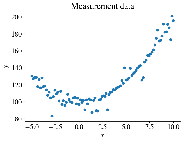
Let’s look again first at numerical regression and generate some synthetic data that are essentially quadratic but with some non-trivial measurement noise. We could also do this for logistic regression/classification, but I think that numerical regression is probably the most familiar to you to appreciate the next steps in this notebook.

Code

nr_measurements=100

x = np.linspace(-5,10,nr_measurements)
y_theoretical = 100 + x**2

y = y_theoretical + (x-5)*np.random.uniform(-1,1,x.shape)
p = np.random.permutation(len(y))
y[p[:25]] = y[p[:25]] + np.random.uniform(-20,20,25)

plt.figure()
plt.title('Measurement data')
plt.scatter(x,y)
plt.xlabel(r'$x$')
plt.ylabel(r'$y$')

measurement_error = mean_squared_error(y_theoretical, y)/2
print("Measurement error is", round(measurement_error,2))

x_save = x
y_save = y

Measurement error is 23.08

Feature engineering: high-order polynomials

In general, we may of course not know what functional form our measured data have. Indeed, we may want to use machine learning tools to find out. Remember that any function can be approximated by a polynomial expansion. For a ‘perfect’ approximation one needs infinite polynomial terms, but usually only a few terms are sufficient for a very good approximation.

To develop a more-or-less universal tool here, let’s try to fit our data with a 15th order polynomial. Remember, we do this by performing a linear regression but using 15 additional features besides the feature \(x_1=x\) itself, namely the bias-feature \(x_0=1\) and all the higher-order terms \(x_2 = x^2\), \(x_3 = x^3\), \(\ldots x_{15} = x^{15}\) (noting that \(x_2\) denotes feature 2, i.e. the subscript indexes features, whereas \(x^2\) here does in fact mean \(x\)-squared, and similar for all the other terms).

For illustrative purposes, I only consider one actual independent variable \(x\) here, but everything below works equally well for multiple distinct features, in which case we would not only generate features of all the powers of individual features but also all the combinations of cross-products (feature 1 squared times feature 2 cubed times feature 3, etc).

Remember that this is an example of what in machine learning is called feature engineering, i.e. generating new features from existing ones. In typical machine learning examples like predicting house prices, you could similarly group together various features that are initially provided separately to see if you can engineer a feature that is a better predictor of house prices. For example, you could combine street-width and depth of property into lot size, divide total square footage by number of rooms to get some sense of whether rooms are large or tiny, combine or separate full bathrooms with just toilets, etc.

Here we go, explicit code (instead of the function we wrote before) to generate the polynomial features, which we combine in our usual feature array, called x_poly again:

Code

poly_order = 15
x_poly = np.ones([nr_measurements,poly_order+1]) # assign memory

for i in range(poly_order+1):
  x_poly[:,i] = x**i

m,n = np.shape(x_poly)

With our convenient function defined above, we should now be able to solve this problem with just one line of code.

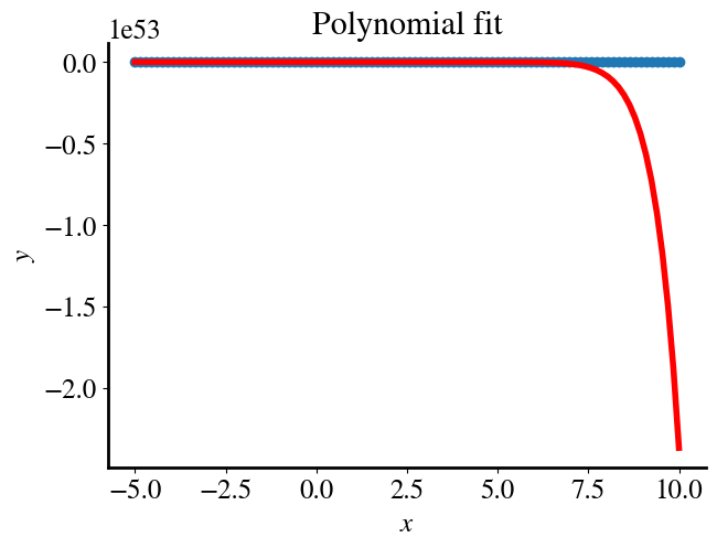
However, you see that the gradient descent algorithm (solver=1) diverges quickly, while the accelerated method (solver=2) converges to some bogus result.

Code

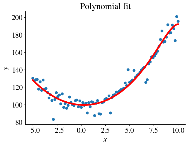
solver = 1 # 1 is our gradient descent, 2 is the accelerated Newton solver we used before

# Do the fitting:
theta_fit = solve_theta(x_poly, y,0.001,0.0001,solver,0)


# Plotting:
y_pred = x_poly.dot(theta_fit)

plt.figure()
plt.title('Polynomial fit')
plt.scatter(x,y)
plt.plot(x,y_pred, color='r', linewidth=4)
plt.xlabel(r'$x$')
plt.ylabel(r'$y$')

GD_error = mean_squared_error(y_pred, y)/2
print("Fitting error is", round(GD_error,2))

1 1.2531328044837041e+50 Errors are diverging: 1.031475131900631e+54 > 8231.171733833933
Problem solved with fitting parameters:

Parameter         Value
      θ_0 -4.085828e+23
      θ_1 -3.873376e+24
      θ_2 -3.684533e+25
      θ_3 -3.515763e+26
      θ_4 -3.363959e+27
      θ_5 -3.226742e+28
      θ_6 -3.102098e+29
      θ_7 -2.988399e+30
      θ_8 -2.884269e+31
      θ_9 -2.788562e+32
     θ_10 -2.700304e+33
     θ_11 -2.618669e+34
     θ_12 -2.542945e+35
     θ_13 -2.472521e+36
     θ_14 -2.406866e+37
     θ_15 -2.345520e+38
Fitting error is 7.492597874104826e+104

What is going on?

The reason is that for our polynomial features of values \(x\) up to \(x=10\), each polynomial features is essentially an order of magnitude more than the last one, and the last points of the \(x_{15}\)-feature are a whopping 15 orders of magnitude larger than the last point of \(x_1=x\) itself, as shown in the first print statement below.

Now, that doesn’t necessarily matter in the end and in principle just means that the fitting parameters \(\theta\) of the highest-order terms, such as \(\theta_{15}\), probably will be about 15 orders of magnitude smaller than than for the first features, e.g. \(\theta_1\).

The problem, though, originates from the fact that the (magnitude of the) gradients in the cost (fitting error) also vary by 15 orders of magnitude in each feature-direction, as shown in the next cell where we compute the error/loss function and its gradients for an initial guess of all \(\theta\) equal to zero:

Code

print("Last row of polynomial feature array:\n", x_poly[-1,:],"\n\n")

n_features = x_poly.shape[1]
initial_theta = np.zeros(n_features)   # starting guess

cost_initial_guess = cost(initial_theta, x_poly, y)
print("Cost for initial guess:\n", np.round(cost_initial_guess,1),"\n\n")

costgradient_initial_guess = gradient(initial_theta, x_poly, y)
print("Cost gradient for initial guess:\n", np.round(costgradient_initial_guess,2),"\n\n")

Last row of polynomial feature array:
 [1.e+00 1.e+01 1.e+02 1.e+03 1.e+04 1.e+05 1.e+06 1.e+07 1.e+08 1.e+09
 1.e+10 1.e+11 1.e+12 1.e+13 1.e+14 1.e+15] 


Cost for initial guess:
 8231.2 


Cost gradient for initial guess:
 [-1.25070000e+02 -4.05120000e+02 -3.94620000e+03 -2.70619200e+04
 -2.40600310e+05 -1.99096990e+06 -1.77576097e+07 -1.56999556e+08
 -1.42502685e+09 -1.29877947e+10 -1.19795050e+11 -1.11117465e+12
 -1.03790063e+13 -9.74199779e+13 -9.18815643e+14 -8.69995732e+15]

In schemes that are some version of gradient descent, each iteration moves a little bit down-hill in each feature dimension. The ‘little bit’ is typically governed by a single learning rate factor \(\alpha\). But if the slope in one direction is 15 orders of magnitude steeper than in another direction, these schemes will move very fast in the former direction and will basically never converge in any of the other directions (features) with orders of magnitude lower slope.

You can visualize this for yourself with physical objects: take/imagine a sheet pan (or piece of carboard or something) and rest one corner on a table such that it is the lowest point and release a marble from the diagonally oposite corner which is the highest point. You want (at least in gradient descent) the marble to roll from the highest to the lowest point along the shortest line diagonally from the highest to the lowest corner points. However, if you tilt the sheet such that it is much steeper in one direction than the other, a marble will first roll down (fast) in the steepest direction and then (slower) along the more gradual slope, together forming a longer L-shaped path. (The width and length of the sheet representing two features.)

You can also see this in the very first module where I introduced gradient descent and showed the gradient descent convergence path on top of the full surface of errors (computed by multiple nested loops). Indeed the errors first moved steeply down (=converged) the direction of one feature (and corresponding \(\theta\)) and then the other.

The same issue occurs (whether or not polynomial features are used) when multiple distict features are used that have very different magnitudes. Even just the use of different units for the same variable could have major effects on a regression algoritm. For instance, if one feature is temperature in Celcius, say between 0 and 100 degrees C, and another feature is pressure, from atmospheric 1 bar to maybe 10 bar, then both features have reasonably similar orders of magnitude. But if, instead, pressures were give in the standard unit of Pascal, then those same values would range between \(10^5\) and \(10^7\) Pascal! In that case, you would likely see that a regression like gradient descent might quickly find the best fitting parameter for the pressure feature, but would never (or only very slowly) converge to a good fit for the temperature.

Feature scaling

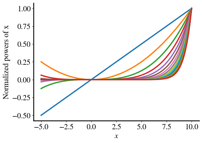
All the aformentioned is a long motivation for the common practice in machine learning to use feature scaling. In the example in this notebook, we simily normalize each feature by its maximum. [In this particular example, this happens to be the last row of the feature array.] We can now divide all the values in each column (feature) by its maximum value, such that each column will range from \(-1<x_i<1\). This is done in the next cell, which then also plots each of the normalized polynomial features versus the original feature \(x_1=x\).

Code


norms = np.amax(x_poly, axis=0)
# Note that this also happens to be the last row in our feature array
# for this particular example, where the x values and all its powers increase
# monotonically, so this would give the same result:
# norms = x_poly[-1,:]


x_poly_norm = x_poly/norms

# Plotting:
plt.plot(x,x_poly_norm[:,1])

for i in range(2,poly_order):
  plt.plot(x,x_poly_norm[:,i])

plt.xlabel(r'$x$')
plt.ylabel('Normalized powers of x');

By working with normalized features, most regression schemes will work much better. In fact, many will not work at all otherwise, and I should emphasize that I had to manipulate some examples in earlier modules to work at all without discussing feature scaling yet.

You can investigate this in much more detail by 1) plotting the cost for each iteration and seeing how well it converges to the minimum cost/error, i.e. whether or not it follows a pretty direct path or is ‘distracted’ by features that result in a steeper cost gradient, or 2) simply plotting the error as a function of number of iterations, which is the learning curve. Doing so for various unnormalized versus normalized features will show you the importance of scaling your features. I think this point is probably abundantly clear, though, and will not explore this any further in actual codes/examples here.

Fitting parameters for normalized versus unnormalized features

When you perform a regression on normalized features, the fitting parameters \(\theta\) that you find will of course be the parameters of a linear combination of those normalized features. If you want to find the parameters of the original non-normalized features, you simply have to divide the fitted \(\theta_i\) by the same normalization factors that were used for each corresponding feature \(x_i\).

To demonstrate why this is so, consider just a single feature \(x_2\). Without normalization, we would find the best \(\theta_2\) to fit \(y = \theta_2 x_2 = \theta_2 x^2\). If, instead, we normalized the feature and indicate the normalization by a tilde, such that \(\tilde{x}_2 = \frac{x^2}{\mathrm{max}(x^2)}\), we would fit \(y = \tilde{\theta}_2 \tilde{x}_2\), where \(\tilde{\theta}_2\) of course is the fitting parameter with respect to the normalized feature \(\tilde{x}_2\). The \(y\) and measurements \(x_2\) are the same in both cases, so we can equate the two expressions to see the relationship between fitted \(\tilde{\theta}_2\) and what the corresponding \(\theta_2\) would be for the unnormalized \(x_2\):

\(y = \tilde{\theta}_2 \tilde{x}_2 = \tilde{\theta}_2 \frac{x^2}{\mathrm{max}(x^2)} = \theta_2 x^2\), such that \(\theta_2 = \frac{\tilde{\theta}_2 }{ \mathrm{max}(x^2)}\).

More generally, features are also often shifted such that they are centered around zero, for instance (for each feature \(i\)) as:

\(\tilde{x}_i = \frac{x_i - \mathrm{mean} (x_i) }{\mathrm{max} (x_i) - \mathrm{min}( x_i )}\),

or always range from \(0<\tilde{x}_i<1\) by (‘min-max’) scaling as:

\(\tilde{x}_i = \frac{x_i - \mathrm{min} (x_i) }{\mathrm{max} (x_i) - \mathrm{min}( x_i )}\).

These shifted scalings make it a bit messier to find the parameters \(\theta\) for the original features, though, so in these examples I only perform feature scaling by a single overall factor for each feature as explained above (note that the data are already centered roughly around 0 anyway).

In the scikit-learn libary, there are various easy-to-use scaling functions that take care of all this, such as StandardScaler, MinMaxScaler, and several others. These can be combined into a preprocession pipeline (https://scikit-learn.org/stable/modules/classes.html#module-sklearn.preprocessing) before solving the actual regression or classification problem.

Another Illustration of Importance of Feature Scaling

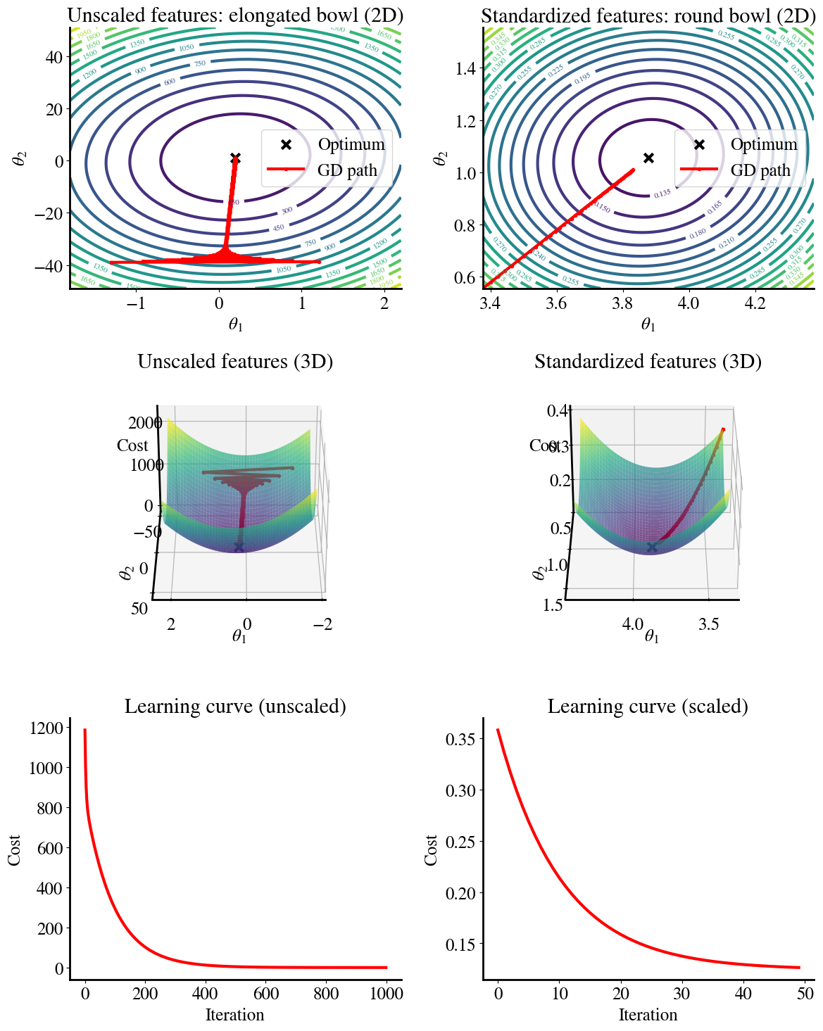
Below is another example of the importance of feature scaling. We consider a simple linear function of two features. One features ranges from \(0<x_2<1\) and the other is just one order of magnitude larger and ranges from \(0<x_1<20)\). We perform linear regression on those ‘raw’ features and for the case where \(x_1\) is normalized, i.e. to the same range as \(x_2\).

The top plots give the error contours (the 2D version of the surface error plots that I showed before). For the scaled features, these contours are perfect circles (with the separation of contours quadratic in each direction). When we start from an initial guess for \(\theta_1\), \(\theta_2\) in the ‘bottom-left corner’, we can see how gradient descent converges perfectly along a straight line to the optimum minimum MSE, which is because the error gradients are the same in each direction.

Conversely, when a feature is not scaled, the circles turn into elongated elipses. Note the different scales of the \(\theta_1\) and \(\theta_2\) axes (in other words, the elipse are much more elongated that the figure suggests)! Now, when we do gradient descent, the gradient in one direction is much larger than in the other direction. So when we take an equal step-size (learning rate) for both \(\theta_1\) and \(\theta_2\), we move primarily along the steepest gradient and don’t really converge in the other direction. This can result in a zig-zagging path that takes many more iterations to get to the best fit.

The second row shows the exact same data but as 3D surface plots instead of flattened 2D contours. This is a nicer visualization close to actual topography that shows the steepness (gradients) more intuitively (though again notice the different ranges of the two axes). You can also see the zig-zagging of gradient descent towards the global minimum, i.e. smallest MSE error, more clearly.

The impact of all this is illustrated in the bottom two figures, which show the learning curves for gradient descent using either ‘raw’/unscaled features on the left or using rescaled features on the right.

You can see that the unscaled feature requires about \(20\times\) more iterations to converge. And I note that this is after tweaking the learning rate to be as high as it can be; making it even higher (e.g. the same as for the scaled feature), it actually doesn’t converge at all.

Code

# --- Synthetic data with scale difference (scaling demo only) ---
from sklearn.preprocessing import StandardScaler

rng = np.random.default_rng(0)
m_scaleDemo = 200
x1_scaleDemo = rng.normal(0, 20, m_scaleDemo)   # larger-scale feature
x2_scaleDemo = rng.normal(0, 1, m_scaleDemo)    # smaller-scale feature
Xraw_scaleDemo = np.c_[x1_scaleDemo, x2_scaleDemo]
theta_true_scaleDemo = np.array([0.2, 1.0])
y_scaleDemo = Xraw_scaleDemo @ theta_true_scaleDemo + rng.normal(0, 0.5, m_scaleDemo)

# Standardized features
scaler_scaleDemo = StandardScaler()
Xstd_scaleDemo = scaler_scaleDemo.fit_transform(Xraw_scaleDemo)

# --- Cost and gradient ---
def cost_and_grad_scaleDemo(theta, X, y):
    m = len(y)
    r = X @ theta - y
    J = 0.5 * (r @ r) / m
    g = X.T @ r / m
    return J, g

# --- Error surface centered on optimum ---
def error_surface_scaleDemo(theta_opt, X, y, span1, span2, n=100):
    t1_range = np.linspace(theta_opt[0]-span1, theta_opt[0]+span1, n)
    t2_range = np.linspace(theta_opt[1]-span2, theta_opt[1]+span2, n)
    T1, T2 = np.meshgrid(t1_range, t2_range)
    J = np.zeros_like(T1)
    for i in range(n):
        for j in range(n):
            th = np.array([T1[i,j], T2[i,j]])
            J[i,j], _ = cost_and_grad_scaleDemo(th, X, y)
    return T1, T2, J

# --- Gradient descent path (also record cost) ---
def gd_path_scaleDemo(X, y, alpha, start, iters=50):
    theta = start.copy()
    path = [theta.copy()]
    costs = []
    for _ in range(iters):
        J, g = cost_and_grad_scaleDemo(theta, X, y)
        costs.append(J)
        theta -= alpha * g
        path.append(theta.copy())
    return np.array(path), np.array(costs)

# --- Compute optima ---
theta_opt_raw_scaleDemo = np.linalg.pinv(Xraw_scaleDemo) @ y_scaleDemo
theta_opt_std_scaleDemo = np.linalg.pinv(Xstd_scaleDemo) @ y_scaleDemo

# --- Error surfaces ---
T1_raw_sD, T2_raw_sD, J_raw_sD = error_surface_scaleDemo(theta_opt_raw_scaleDemo, Xraw_scaleDemo, y_scaleDemo, span1=2.0, span2=50)
T1_std_sD, T2_std_sD, J_std_sD = error_surface_scaleDemo(theta_opt_std_scaleDemo, Xstd_scaleDemo, y_scaleDemo, span1=0.5, span2=0.5)

# --- Gradient descent paths + learning curves ---
theta_start_raw_scaleDemo = theta_opt_raw_scaleDemo + np.array([-1.5, -40])
theta_start_std_scaleDemo = np.array([T1_std_sD.min(), T2_std_sD.min()])

path_raw_sD, costs_raw_sD = gd_path_scaleDemo(Xraw_scaleDemo, y_scaleDemo, alpha=0.005, start=theta_start_raw_scaleDemo, iters=1000)
path_std_sD, costs_std_sD = gd_path_scaleDemo(Xstd_scaleDemo, y_scaleDemo, alpha=0.05, start=theta_start_std_scaleDemo, iters=50)

# --- Plot: 3 rows (2D contours, 3D surfaces, learning curves) ---
fig = plt.figure(figsize=(12,15))

# Row 1: 2D contours
ax1 = fig.add_subplot(3,2,1)
cs1 = ax1.contour(T1_raw_sD, T2_raw_sD, J_raw_sD, levels=20)
ax1.clabel(cs1, inline=1, fontsize=8)
ax1.scatter(*theta_opt_raw_scaleDemo, c='black', marker='x', s=80, label="Optimum")
ax1.plot(path_raw_sD[:,0], path_raw_sD[:,1], 'o-r', markersize=3, label="GD path")
ax1.set_title("Unscaled features: elongated bowl (2D)")
ax1.set_xlabel(r"$\theta_1$")
ax1.set_ylabel(r"$\theta_2$")
ax1.legend()

ax2 = fig.add_subplot(3,2,2)
cs2 = ax2.contour(T1_std_sD, T2_std_sD, J_std_sD, levels=20)
ax2.clabel(cs2, inline=1, fontsize=8)
ax2.scatter(*theta_opt_std_scaleDemo, c='black', marker='x', s=80, label="Optimum")
ax2.plot(path_std_sD[:,0], path_std_sD[:,1], 'o-r', markersize=3, label="GD path")
ax2.set_title("Standardized features: round bowl (2D)")
ax2.set_xlabel(r"$\theta_1$")
ax2.set_ylabel(r"$\theta_2$")
ax2.legend()

# Row 2: 3D surfaces
ax3 = fig.add_subplot(3,2,3, projection='3d')
ax3.plot_surface(T1_raw_sD, T2_raw_sD, J_raw_sD, cmap="viridis", alpha=0.7)
ax3.scatter(*theta_opt_raw_scaleDemo, cost_and_grad_scaleDemo(theta_opt_raw_scaleDemo,Xraw_scaleDemo,y_scaleDemo)[0], c='black', marker='x', s=80, label="Optimum")
ax3.plot(path_raw_sD[:,0], path_raw_sD[:,1],
         [cost_and_grad_scaleDemo(th,Xraw_scaleDemo,y_scaleDemo)[0] for th in path_raw_sD],
         'o-r', markersize=3, label="GD path")
ax3.set_title("Unscaled features (3D)")
ax3.set_xlabel(r"$\theta_1$")
ax3.set_ylabel(r"$\theta_2$")
ax3.set_zlabel("Cost")
ax3.view_init(elev=30, azim=90)

ax4 = fig.add_subplot(3,2,4, projection='3d')
ax4.plot_surface(T1_std_sD, T2_std_sD, J_std_sD, cmap="viridis", alpha=0.7)
ax4.scatter(*theta_opt_std_scaleDemo, cost_and_grad_scaleDemo(theta_opt_std_scaleDemo,Xstd_scaleDemo,y_scaleDemo)[0], c='black', marker='x', s=80, label="Optimum")
ax4.plot(path_std_sD[:,0], path_std_sD[:,1],
         [cost_and_grad_scaleDemo(th,Xstd_scaleDemo,y_scaleDemo)[0] for th in path_std_sD],
         'o-r', markersize=3, label="GD path")
ax4.set_title("Standardized features (3D)")
ax4.set_xlabel(r"$\theta_1$")
ax4.set_ylabel(r"$\theta_2$")
ax4.set_zlabel("Cost")
ax4.view_init(elev=30, azim=90)

# Row 3: Learning curves
ax5 = fig.add_subplot(3,2,5)
ax5.plot(costs_raw_sD, 'r-')
ax5.set_title("Learning curve (unscaled)")
ax5.set_xlabel("Iteration")
ax5.set_ylabel("Cost")

ax6 = fig.add_subplot(3,2,6)
ax6.plot(costs_std_sD, 'r-')
ax6.set_title("Learning curve (scaled)")
ax6.set_xlabel("Iteration")
ax6.set_ylabel("Cost")

plt.tight_layout()
plt.show()

Fit scaled polynomial features

Now that you know about feature engineering together with feature scaling, let’s apply this to the problem at hand. Again, we use our handy general solver function, pick the accelerated Newton method and a tight tolerance (requiring an accuracy of \(10^{-3}\)), and using normalized polynomial features up to 15 orders.

[As an aside, if you change the tolerance below to much smaller values of \(10^{-5}\), interestingly you will see that the accelerated method will not converge. My solve_theta has a ‘fail-safe’, though, to then try my own hard-coded gradient descent method instead. The latter is much slower but does converge in this case. Almost certainly that means that the accelerated method should also work but may have some default parameters (like the maximum number of iterations allowed) that would need to be tuned.]

Code

tol = 1e-4
solver = 1

theta_fit_norm = solve_theta(x_poly_norm, y,1,tol,solver,0)

Problem solved with fitting parameters:

Parameter     Value
      θ_0 99.606204
      θ_1 -5.602790
      θ_2 98.167670
      θ_3  2.901160
      θ_4 21.390176
      θ_5 -1.408059
      θ_6  2.262976
      θ_7 -2.868100
      θ_8 -2.190368
      θ_9 -3.351911
     θ_10 -3.175410
     θ_11 -3.319178
     θ_12 -3.084464
     θ_13 -2.840911
     θ_14 -2.439752
     θ_15 -1.972753

The fitted \(\tilde{\theta}\) values found by the numerical regression machine learning algorithm (which minimizes the cost function) are still for the normalized features. Below, we calculate the corresponding \(\theta\) with respect to the unnormalized features, compute predictions \(y = \theta x\), print the fitting error, and plot the fitted result.

Code

theta_fit= theta_fit_norm/norms
print("Fitting parameters for original/unscaled features are:\n", theta_fit)

#Prediction:
y_pred = x_poly.dot(theta_fit)

#Plotting:
plt.figure()
plt.title('Polynomial fit')
plt.scatter(x,y)
plt.plot(x,y_pred, color='r', linewidth=4)
plt.xlabel(r'$x$')
plt.ylabel(r'$y$')

GD_error = mean_squared_error(y_pred, y)/2
print("Fitting error is", round(GD_error,2))

Fitting parameters for original/unscaled features are:
 [ 9.96062038e+01 -5.60278971e-01  9.81676701e-01  2.90116003e-03
  2.13901757e-03 -1.40805922e-05  2.26297621e-06 -2.86809961e-07
 -2.19036822e-08 -3.35191114e-09 -3.17541045e-10 -3.31917780e-11
 -3.08446377e-12 -2.84091133e-13 -2.43975217e-14 -1.97275312e-15]
Fitting error is 21.83

If you compare the fitting error to the ‘measurement’ error, which is the artificially introduced noise in the data, you’ll notice that the fitting error is actually less than that. This is a first indication that a 15th order polynomial may be ‘overkill’ and we are overfitting our data. Avoiding this overfitting is the main subject of this module.

Note on Black Box (optional aside)

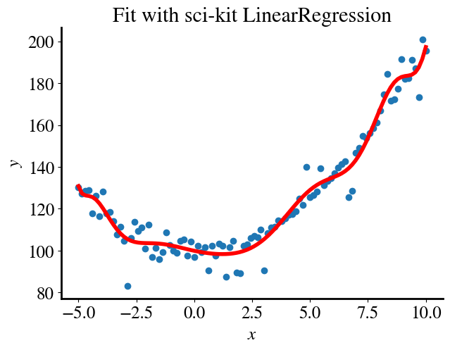
Before elaborating on the main topic of regularization, one other interesting observation: If instead of our own Gradient Descent method or its accelerated Newton method (solver = 1 or 2), we use the scikit-learn LinearRegression solver (solver=5 in my solve_theta function), we find this:

Code

tol = 1e-5
solver = 5

theta_blackbox_norm = solve_theta(x_poly_norm, y,1,tol,solver,0)

theta_blackbox = theta_blackbox_norm/norms
print("Fitting parameters for unscaled features are:\n", theta_blackbox)

y_pred = x_poly.dot(theta_blackbox)

plt.figure()
plt.title('Fit with sci-kit LinearRegression')
plt.scatter(x,y)
plt.plot(x,y_pred, color='r', linewidth=4)
plt.xlabel(r'$x$')
plt.ylabel(r'$y$')

BB_error = mean_squared_error(y_pred, y)/2
print("Fitting error is", round(BB_error,2))

Problem solved with fitting parameters:

Parameter         Value
      θ_0  9.993863e+01
      θ_1 -2.342505e+01
      θ_2  6.310878e+01
      θ_3  2.720494e+02
      θ_4 -1.273853e+03
      θ_5  3.464456e+03
      θ_6  1.765338e+04
      θ_7 -6.435416e+04
      θ_8 -8.637692e+03
      θ_9  2.486206e+05
     θ_10 -3.587900e+05
     θ_11  5.752833e+04
     θ_12  6.241464e+05
     θ_13 -1.110950e+06
     θ_14  8.146342e+05
     θ_15 -2.222564e+05
Fitting parameters for unscaled features are:
 [ 9.99386291e+01 -2.34250532e+00  6.31087840e-01  2.72049382e-01
 -1.27385284e-01  3.46445600e-02  1.76533793e-02 -6.43541633e-03
 -8.63769155e-05  2.48620649e-04 -3.58790036e-05  5.75283340e-07
  6.24146383e-07 -1.11094965e-07  8.14634165e-09 -2.22256381e-10]
Fitting error is 17.25

the error is even lower and the fit even ‘better’, both of which mean that there is even more overfitting. The point I want to make, though, is that it is not really clear why the LinearRegression function results in such a different fit.

Related: if you try to fit the unnormalized features with the LinearRegression solver=5 , you’ll see that it does readily fit those without problems and with the exact same fitting parameters and final error.

Most likely, for robustness and user-friendliness, LinearRegression always performs feature scaling as well as perhaps centering around zero, automatically and internally for better performance.

There is nothing necessarily bad about any of the above, except the unease of an academic/scientist at seeing results like this without being able to fully explain them. This is of course always the downside of a ‘black box’ model compared to, e.g., a gradient descent code in this context, that you can code and fully understand yourself. At least in this case, python and scikit-learn are all open source and with enough determination one could find out exactly how their algorithms are implemented.

Exploring Overfitting

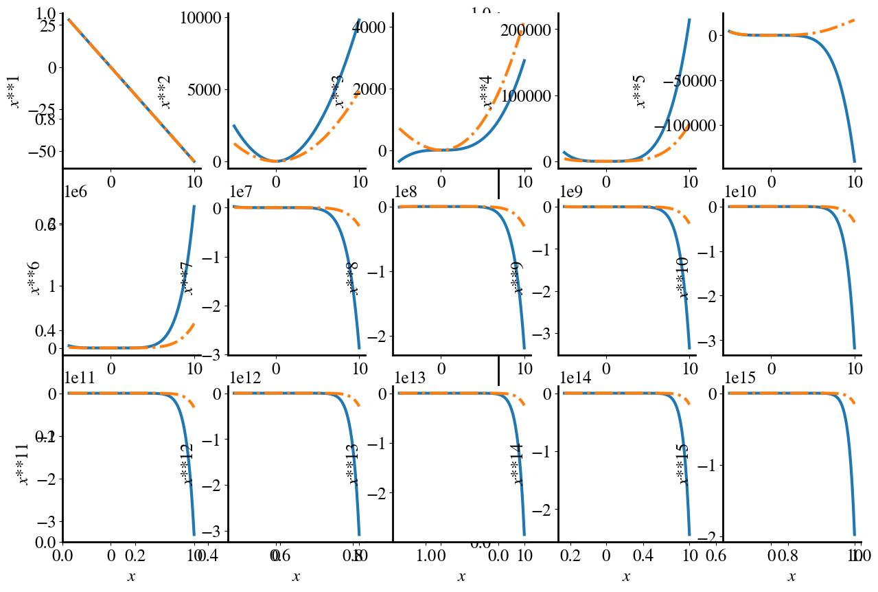
Below, I plot the contribution of each individual polynomial term (except the bias \(\theta_0\)), as well as (dash-dotted line) the sum of all the terms up to that order (i.e., panel 3 shows \(\theta_3* x^3\) in solid and \(\theta_1 x_1+\theta_2 x_2 + \theta_3 x_3\) in dash-dotted line). To have both individual feature contributions and the sum of all contributions on a similar scale, the sum of terms up to order \(n\) is divided by \(n\).

Code

plt.subplots(1,2,figsize=(15,10))
for i in range(poly_order):
  plt.subplot(3,5,i+1)
  yi = theta_fit_norm[i+1]*x_poly[:,i+1]
  y_cum = x_poly[:,1:i+2].dot(theta_fit_norm[1:i+2])/(i+1)
  plt.plot(x,yi)
  plt.plot(x,y_cum,'-.')
  plt.xlabel(r'$x$')
  j = i+1
  plt.ylabel(r'$x$**'+str(j))
plt.tight_layout()

/tmp/ipython-input-2561520125.py:11: UserWarning: tight_layout not applied: number of columns in subplot specifications must be multiples of one another.
  plt.tight_layout()

The take-away point from this illustration is that all terms, all the way up to \(\theta_{15}x^{15}\) contribute significantly to this polynomial fit, even though we ‘know’ that the synthetic data are really only second-order. This means that we are over-fitting the data, i.e. have too much model complexity.

Next week, we’ll explore in detail how to avoid both underfitting and overfitting through, what’s called, regularization. Underfitting is closely related to the bias of a model and overfitting to its variance. In the process, you’ll also learn about cross-validation.

In this week’s lab, you’ll also learn and practice more with topics covered in the lecture related to data preprocessing pipelines, such as turning categorical string values of features into numbers with one-hot-encoding and filling in missing (or NaN) values with impute.

✏️ Next up: Practice: ML Pipelines

📖 Next module: Module 6: Cross-Validation & Regularization