Which platform should I choose?

📖 Review the Lecture notes

Multivariate Linear Regression

Summary & Objective

In this lab you will explore applying multivariate linear regression. We’ll step away from Sciences and Engineering applications and play around with a typical machine learning problem: predicting real estate house prices from historical data. The lab offers the opportunity to do linear regression with either ‘black box’ scikit-learn functions and/or the gradients descent algorithm that was presented in detail in the lectures.

Load libraries

As always, we start by plugging in some essential python libraries. The same ones you used last week.

import numpy as np
import matplotlib.pyplot as plt
import pandas as pd
import requests
import csv
from sklearn.linear_model import LinearRegression
from sklearn.metrics import mean_absolute_error,mean_squared_error,r2_score

Load data

Again, we’ll import a file of ‘measurement’ data directly from the internet without saving it on your local computer or google drive. This process is a bit non-trivial, so I’ll provide the code. I encourage you to also just copy the same URL into your browser and download the file to your computer so you can inspect it. You can import this tab-delimited file into a spreadsheet program like Excel to perhaps more easily inspect what these data look like. I also uploaded the data file to Carmen (mostly for myself in case the link ever goes dead).

file_url = 'http://jse.amstat.org/v19n3/decock/AmesHousing.txt'

r = requests.get(file_url);
open('AmesHousing.txt', 'wb').write(r.content);

Next, load the data in to a pandas dataframe so we can manipulate it in python:

df = pd.read_csv('AmesHousing.txt',sep='\t',header=(0))

As before, you can use .head() to see the first rows of the dataframe, which also shows the column headers:

df.head()

	Order	PID	MS SubClass	MS Zoning	Lot Frontage	Lot Area	Street	Alley	Lot Shape	Land Contour	...	Pool Area	Pool QC	Fence	Misc Feature	Misc Val	Mo Sold	Yr Sold	Sale Type	Sale Condition	SalePrice
0	1	526301100	20	RL	141.0	31770	Pave	NaN	IR1	Lvl	...	0	NaN	NaN	NaN	0	5	2010	WD	Normal	215000
1	2	526350040	20	RH	80.0	11622	Pave	NaN	Reg	Lvl	...	0	NaN	MnPrv	NaN	0	6	2010	WD	Normal	105000
2	3	526351010	20	RL	81.0	14267	Pave	NaN	IR1	Lvl	...	0	NaN	NaN	Gar2	12500	6	2010	WD	Normal	172000
3	4	526353030	20	RL	93.0	11160	Pave	NaN	Reg	Lvl	...	0	NaN	NaN	NaN	0	4	2010	WD	Normal	244000
4	5	527105010	60	RL	74.0	13830	Pave	NaN	IR1	Lvl	...	0	NaN	MnPrv	NaN	0	3	2010	WD	Normal	189900

5 rows × 82 columns

In this case, perhaps even more useful is to use .info()

df.info()

<class 'pandas.core.frame.DataFrame'>
RangeIndex: 2930 entries, 0 to 2929
Data columns (total 82 columns):
 #   Column           Non-Null Count  Dtype  
---  ------           --------------  -----  
 0   Order            2930 non-null   int64  
 1   PID              2930 non-null   int64  
 2   MS SubClass      2930 non-null   int64  
 3   MS Zoning        2930 non-null   object 
 4   Lot Frontage     2440 non-null   float64
 5   Lot Area         2930 non-null   int64  
 6   Street           2930 non-null   object 
 7   Alley            198 non-null    object 
 8   Lot Shape        2930 non-null   object 
 9   Land Contour     2930 non-null   object 
 10  Utilities        2930 non-null   object 
 11  Lot Config       2930 non-null   object 
 12  Land Slope       2930 non-null   object 
 13  Neighborhood     2930 non-null   object 
 14  Condition 1      2930 non-null   object 
 15  Condition 2      2930 non-null   object 
 16  Bldg Type        2930 non-null   object 
 17  House Style      2930 non-null   object 
 18  Overall Qual     2930 non-null   int64  
 19  Overall Cond     2930 non-null   int64  
 20  Year Built       2930 non-null   int64  
 21  Year Remod/Add   2930 non-null   int64  
 22  Roof Style       2930 non-null   object 
 23  Roof Matl        2930 non-null   object 
 24  Exterior 1st     2930 non-null   object 
 25  Exterior 2nd     2930 non-null   object 
 26  Mas Vnr Type     1155 non-null   object 
 27  Mas Vnr Area     2907 non-null   float64
 28  Exter Qual       2930 non-null   object 
 29  Exter Cond       2930 non-null   object 
 30  Foundation       2930 non-null   object 
 31  Bsmt Qual        2850 non-null   object 
 32  Bsmt Cond        2850 non-null   object 
 33  Bsmt Exposure    2847 non-null   object 
 34  BsmtFin Type 1   2850 non-null   object 
 35  BsmtFin SF 1     2929 non-null   float64
 36  BsmtFin Type 2   2849 non-null   object 
 37  BsmtFin SF 2     2929 non-null   float64
 38  Bsmt Unf SF      2929 non-null   float64
 39  Total Bsmt SF    2929 non-null   float64
 40  Heating          2930 non-null   object 
 41  Heating QC       2930 non-null   object 
 42  Central Air      2930 non-null   object 
 43  Electrical       2929 non-null   object 
 44  1st Flr SF       2930 non-null   int64  
 45  2nd Flr SF       2930 non-null   int64  
 46  Low Qual Fin SF  2930 non-null   int64  
 47  Gr Liv Area      2930 non-null   int64  
 48  Bsmt Full Bath   2928 non-null   float64
 49  Bsmt Half Bath   2928 non-null   float64
 50  Full Bath        2930 non-null   int64  
 51  Half Bath        2930 non-null   int64  
 52  Bedroom AbvGr    2930 non-null   int64  
 53  Kitchen AbvGr    2930 non-null   int64  
 54  Kitchen Qual     2930 non-null   object 
 55  TotRms AbvGrd    2930 non-null   int64  
 56  Functional       2930 non-null   object 
 57  Fireplaces       2930 non-null   int64  
 58  Fireplace Qu     1508 non-null   object 
 59  Garage Type      2773 non-null   object 
 60  Garage Yr Blt    2771 non-null   float64
 61  Garage Finish    2771 non-null   object 
 62  Garage Cars      2929 non-null   float64
 63  Garage Area      2929 non-null   float64
 64  Garage Qual      2771 non-null   object 
 65  Garage Cond      2771 non-null   object 
 66  Paved Drive      2930 non-null   object 
 67  Wood Deck SF     2930 non-null   int64  
 68  Open Porch SF    2930 non-null   int64  
 69  Enclosed Porch   2930 non-null   int64  
 70  3Ssn Porch       2930 non-null   int64  
 71  Screen Porch     2930 non-null   int64  
 72  Pool Area        2930 non-null   int64  
 73  Pool QC          13 non-null     object 
 74  Fence            572 non-null    object 
 75  Misc Feature     106 non-null    object 
 76  Misc Val         2930 non-null   int64  
 77  Mo Sold          2930 non-null   int64  
 78  Yr Sold          2930 non-null   int64  
 79  Sale Type        2930 non-null   object 
 80  Sale Condition   2930 non-null   object 
 81  SalePrice        2930 non-null   int64  
dtypes: float64(11), int64(28), object(43)
memory usage: 1.8+ MB

As you can see, this gives you the number and the (string) name of each column, but it also provides some other useful information in the context of this exercise.

The 3rd column gives you the number of ‘non-null’ values in each column. A spreadsheet like this (and also Devin Smith’s data last week if you look at the full spreadsheet) can have empty cells, typically when some information is not available for certain measurements. In this case, you can see for instane that only 572 of the 2930 houses have information in the ‘Fence’ column. When you load such data into a pandas dataframe, the value of such cells is NaN, which stands for Not-A-Number. Obviously, ‘not a number’ is not what you want when doing numerical calculations (more on how to fix that below).

Finally, the 4th column tells you the data type of each column. int64 means numerical integer values, which we can work with. ‘Object’ are text (string) values. You can see this in the df.head() results above. The column ‘Street’, for example has values like ‘Pave’. There are ways to turn such categories into numerical values (part of ‘feature engineering’) but that’s a beyond the scope of this exercise (we’ll look at feature engineering in more detail in a later lab).

df['Street']

	Street
0	Pave
1	Pave
2	Pave
3	Pave
4	Pave
...	...
2925	Pave
2926	Pave
2927	Pave
2928	Pave
2929	Pave

2930 rows × 1 columns

dtype: object

As you can see, this dataset has 80 different features for 2930 different houses (‘measurements’), so a great example for multivariate regressions.

[Note that I don’t exactly know what each feature is, but you can mostly guess or probably find it online for the Ames housing dataset.]

Feature selection

Now we get to the fun part. Let’s ‘engineer’ the features that we think are helpful to predict the sale price of each house, which is in the last column. In this exercise we will only explore the ‘hypothesis’ that the sale prices have a linear dependence on the various features in this database (which in this case are indeed ‘features’ of each house).

I will try to just give you enough skeleton code so you don’t get too bogged down in pandas/numpy syntax. The challenge of this lab is for you to come up with the best multivariate linear regression model to predict house prices from whatever combination of features you choose.

To get started, first pull out the last column of the spreadsheet/pandas dataframe, which is the house price. Also, we turn this straight into a numpy array.

y = df['SalePrice'].to_numpy()

It never hurts to visualize what we’re doing to gain some insight. For example, we can look at a histogram plot of house prices (i.e. number of houses sold within bins of certain price ranges):

plt.hist(y);
plt.title('Histogram of house prices')
plt.xlabel('Sale price')
plt.ylabel('# of houses at price');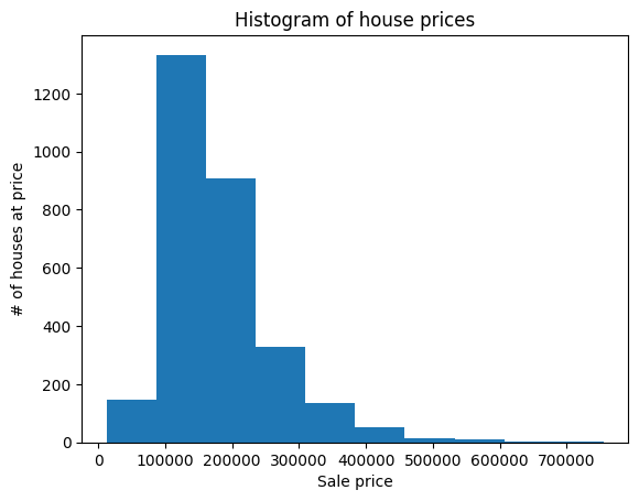

This shows that by fast the most houses are sold around the $100,000 - $200,000 range with a long tail of more expensive houses. The distribution is rather skewed and the numbers are very large. For reasons I won’t go into, it may work better to fit to the (natural) log of house prices instead (but feel free to experiment with both!).

y = np.log(y)

plt.hist(y);
plt.title('Histogram of (log) house prices')
plt.xlabel('Log of sale price')
plt.ylabel('# of houses at price');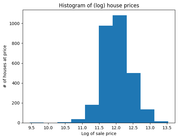

You can see that this looks less skewed (technically: more like a log-normal distribution of data, which is good).

Next we get to the more interesting, an interactive, part of the exercise: selecting the features that you think are helpful in precising sale prices. I will get you started with just 2 (not very good) features to show you how to do this in python, and then let you experiment with as many features as you like. After all, that’s what you gained by now understanding multivariate linear regression.

The goal is to come up with the best combination of features to predict house prices, which we will measure by the R2 score of the final fit, as compared to the actual sale price (which are the labels in our supervised learning approach).

features_i_want = ['Garage Area','Pool Area']

x = df[features_i_want].to_numpy()

x[np.isnan(x)] = 0 # try to understand this nice concise way in which python does this: np.isnan(x) gives the indices where x=NaN and x[np.isnan(x)] then sets just those values to zero

Two notes here:

1. You can see that I do select features by name here, but you could also look back at your previous lab to see how you can select by column number instead to avoid any typos in the column names (seems like less of a concern in this database).
2. In the last line of the code cell above, I set all the potential NaN (not a number) values of empty cells to zero. This will make everything numerical and not result in python errors. However, it is not really the smartest way of doing this. Just because some piece of information is not avialable for some houses (say, basement size), doesn’t mean it is zero, so this could give you weird outliers. A better way is, for example, to set empty cells to the average or mean of all the houses for which that information is available. This requires a bit more numpy familiarity, which you may or may not have yet (of course, try if you’re up to it!)

Next, we’ll use the same tricks as in the last lab to split our data into 80% of the houses as training data and 20% that we will use to validate our models.

nr_data_points, nr_features = np.shape(x)

# splitat is just a variable name that I defne, which we then assign the value of 0.8 times the total number of measurements
# of course 0.8*nr_data_points could be something like 2929.7, so we have to turn that into an integer by rounding up/down
splitat = int(0.8*nr_data_points)

print("Total number of data points", nr_data_points, 'split into ',splitat ,'training data and ',nr_data_points - splitat , 'validation data.' )

Total number of data points 2930 split into  2344 training data and  586 validation data.

# train, validation set split
x_trn, x_val = x[:splitat,:], x[splitat:,:]
y_trn, y_val = y[:splitat,None], y[splitat:,None]

# The above is an elegant short notation to do this, but it is the same as doing it one at a time like:
# x_trn = x[:splitat,:]
# x_val = x[splitat:,:]
# and the same for y_try and y_val, using basic subsetting of the arrays by indices
# This is also short-hand notation for the even more explicit notation:
# x_trn = x[0:splitat,0:nr_features]
# x_val = x[splitat:nr_data_points,0:nr_features]
# where the first index is for the rows, which corresponds to the number of measurement points nr_data_points
# and the second index is for the columns, which are the features.

# Play around with this if it is not clear, and maybe try, e.g., np.shape(x_trn) or print the entire arrays to see what they look like

Note in the above that the features are already a 2D/rank-2 array, and by using the funny ‘None’ notation we also turn the target \(y\) into an actual array with just 1 column (again, this is something peculiar to python that is different from Matlab).

When we deal with many features, it is no longer straightforward to visualize how our target (\(y =\) house prices) plots as a function of multiple variables. You can of course just plot the dependence on one feature at a time to see if the relation already looks linear at all:

plt.scatter(x_trn[:,1],y_trn); # x_trn[:,1] means all measurements (rows) of feature 1 (starting from zero!)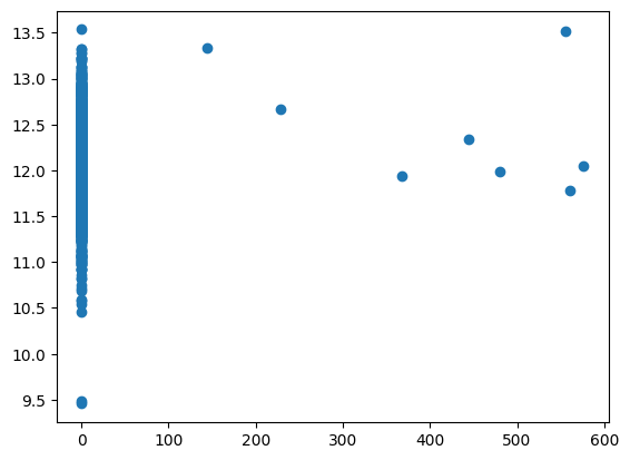

Mostly, what this will show is that each individual feature is not a good linear predictor of sale price. In fact, you’ll likely see so much spread that even any polynomial regression in a single feature will also not be a good model/hypothesis.

Now that we have features and targets defined, and we have our linear hypothesis, we can do the actual regression = model fitting. Note that the code to do this is identical to last week for a single feature (univariate regression).

linear_regression_model = LinearRegression().fit(x_trn, y_trn)

The all-important metric to see how well you did is the fitting error. We could use various metrics, like MSE mean-squared-error, but let’s consider R2 score throughout this exercise. A R2 score of one is perfect and zero is bad, so we want to get as close to 1 as possible.

To be very clear: the linear regression model still minimizes MSE as our cost/lost/error function to find the best fitting parameters. But because MSE is not normalized it is not the most intuitive to see whether a fit is ‘good’ or not. So we also compute R2 after the fact (after fitting) as another measure of how good our fits are.

r2_train = linear_regression_model.score(x_trn,y_trn)
r2_train

0.41711636883613523

If you didn’t modify my code yet, the R2 score is probably not great. Your job is to engineer your own features to improve this.

Btw, just like last week, you can of course also print out the actual fitting parameters for the intercept and the slopes for each of your features:

slope = linear_regression_model.coef_
intercept = linear_regression_model.intercept_

print("Fitting coefficients are slope:", np.round(slope,5), 'and intercept', np.round(intercept,2) )

Fitting coefficients are slope: [[ 1.22e-03 -1.00e-05]] and intercept [11.45]

And one way to get some visual sense of how your model is performing is to plot your predicted house price versus the true house price. If the model is good (high R2 score) these should fall onto a straight 1-to-1 line, and the more scatter you see, the poorer your model performance.

Note that I suggested to fit to the natural logarithm of prices instead of the prices themselves, so to make a plot of the actual prices I plot the exponent of our predicted target \(y\).

house_price_predictions_training = linear_regression_model.predict(x_trn)

plt.scatter(np.exp(y_trn),np.exp(house_price_predictions_training))
plt.plot(np.exp(y_trn),np.exp(y_trn));

plt.title('Predicted vs actual house prices')
plt.xlabel('Actual house price')
plt.ylabel('Predicted house price');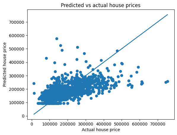

Validation

Of course the last few steps only evaluated the accuracy in fitting the training data, but a more rigorous test of how well your model performs is to see how well it can predict the prices of houses what were not themselves included in the training dataset, i.e., our 20% hold-out measurements of validation data.

house_price_predictions_val = linear_regression_model.predict(x_val)

r2_val = r2_score(house_price_predictions_val, y_val )
print("R2 accuracy on validation data is", r2_val)

R2 accuracy on validation data is -0.3455366678167169

If you haven’t changed any of the above code yet, you might see that this R2 value is even negative, which is a bad fit indeed.

We can again plot the correlation between predicted house prices on the validation data versus our labeled ‘ground truth’ house prices for those same houses.

plt.scatter(np.exp(y_val),np.exp(house_price_predictions_val))
plt.plot(np.exp(y),np.exp(y));

plt.title('Predicted vs actual house prices')
plt.xlabel('Actual house price')
plt.ylabel('Predicted house price');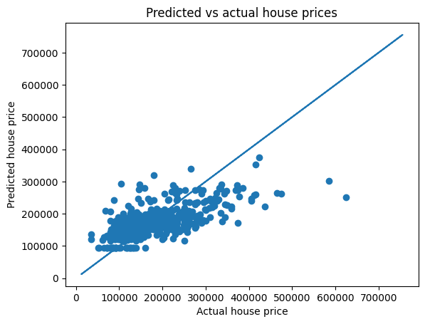

Smart feature engineering

As you may have tried out already, you are likely to initially get to the best linear regression results by throwing the entire ‘kitchen sink’ at it, and including all (numerical) house features. More information is always better right? Well, this is not necessarily entirely true.

First, some features are highly correlated. The square footage on the second floor is perhaps often nearly the same as that of the first floor. It may not hurt, in terms of R2 scores of your fit, to include both, but it won’t help either and you’re making your model unnecessarily complex and more computationally expensive. Ideally, of course you’d like to predict your target (in this case house prices) with the minimum amount of information that is the most important.

Second, it is possible to construct/engineer features that are likely to be more useful than the raw data. For example, we have columns for the year each house was built and the year it was sold (an important point: not all houses were sold in the same year!). The age of the house when it was sold may be a more meaningful predictor, so you would design a feature that is the difference between those two columns.

Third, outliers can really mess up your regression. If you have just a few houses that cost millions of dollars, or were sold extremely cheaply (perhaps because of a foreclosure), this can tilt your entire linear fit in a wrong direction. You are likely more interested in predicting the sale price of the other 97% of houses, say, as accurately as you can, so it can be worth excluding, say, 3% of weird outliers.

In this example, as in most Science/Engineering-related problems, it is generally good to not just use machine learning in a ‘brute force’ type of way and hope for the best, but also insert your own ‘domain knowledge’ to apply machine learning in more clever ways.

Of course, doing some of the above, like combining two features into one, requires a bit more numpy manipulations, but this can be a good exercise.

I really need to make/repeat another important point: using packaged functions like scikit-learn LinearRegression is great in its convenience, but tricky because you really don’t know how they work (again, a black box). You will explore this a bit in the section below in which you will model the same problem with our own gradient descent method, coded from scratch, and you can see it’s actually hard to reproduce the same results.

When you try and do this from scratch, you get a better appreciation of how these machine learning models work.

Without black box (optional, for those interested)

Before modeling multivariate linear (or non-linear) regression from scratch I need to expand on one important point that I likely didn’t have time for in the lecture(s): feature scaling. The explanation is a bit long, so perhaps read outside of class time.

When we have different independent variables (features), each of those features can easily have wildly different (orders of magnitude) ranges of values, even if only by our choice of units. For example: we might have temperature ranging from 50\(^\circ\)F to 90\(^\circ\)F (and not too different in Celcius), and pressures that range either from 1 to 100 bar or (identical, but different unit) 100,000 to 10 million Pascal, and, say, a let’s say an air density of 0.07 when measured in pounds per cubic feet. Or in the example considered in this exercise, we have lot sizes that range from 1,000 to 250,000 square feet, but built/sold years over a range of no more than 100 years.

As a result, the derivatives, or gradients, that we use in the gradient descent method can also have wildly different orders of magnitude in each feature direction. If we use the same learning rate for each feature, in other words we take an equal-sized step ‘down-hill’ allong the error in each feature, we may quicky find the best fit in one feature (with the biggest error slope) but require orders-of-magnitude more steps to find the minimum error for another feature (with a more gradual slope).

The gradient descent method relies on the gradient/slope of the error as a function of fitting parameters, but let me try and give you an even easier example of what I’m trying to get at, a pretty stupid example: Let’s say we took a spreadsheet with 2 identical columns, each of which had pressures ranging from 0 to 100 bar. The actual numbers in the spreadsheet would just be 0, 1, 2, … 100. We could do a univariate linear regression of the second column as the target and the first one as the feature, so we should find a slope of 1. Perhaps we try the brute-force approach of starting with a slope of 0 and then trying slopes of 0.1, 0.2, 0.3 etc until we have a good fit. Or we try gradient descent with a learning rate of 0.1. In both cases it would take <=10 steps to find the best fit. Now consider that we only change the unit of the feature to Pascal (but leave the target the same), so its numerical values are 100,000 to 10,000,000. In this case the ‘true’ slope would be \(10^{-5}\) and if we tried the same step sizes as above, we would completely miss the best fit. Conversely, if we changed the target column to Pascal and left the feature in bars and we used the same step sizes, the true slope would be \(10^5\), so with step sizes of 0.1 it would take a million steps, instead of 10, to find the best fit.

This is a long way of saying: when applying linear or non-linear regression to multipe variables, it is important to rescale those variables (features) to be in a similar range. This helps to have the error gradients also be of similar range and for gradient-descent-type methods to converge efficiently.

Black box functions like LinearRegression do this internally, but if we want to solve the problem from scratch, we also have to do this ourselves.

The common approach is to use so-called ‘min-max’ feature scaling (see, e.g., wikipedia). For each feature \(x\) we take its minimum (np.min(x)) and maximum (np.max(x)) value and define \[ x^\prime = \frac{x-x_\mathrm{min}}{x_\mathrm{max}-x_\mathrm{min}},\] which will turn each feature into values between 0 and 1.

Doing this rescaling can majorly improve the regression / gradient descent efficiency. It does complicate matters a little, though:

1. The best fitting parameters, \(\theta\), from your linear regression will be for the rescaled features, and not your original features. So if you want to express your linear model in terms of those original features, you have to rescale your \(\theta\) accordingly (by one-over the factor that you used to rescale your feature).
2. When you have separate training and validation data, you should make sure to use a consistent rescaling factor for both.

I’ll try and provide an example in a future notebook/lab or lecture, but for now you could try to experiment a little yourself.

Important note on all the above: almost certainly, scikit-learn LinearRegression does this type of feature scaling (and re-scaling of fitting parameters \(\theta\) in the end) internally, or none of the optimization/machine learning algorithms would work.

You may or may not have noticed that LinearRegression also doesn’t require you to have a bias feature \(x_0=1\) to allow for efficient vectorization. This is also likely added internally.

If we wan’t to code linear regression from scratch, we have to do all these steps ourselves (but we can of course turn this into a neat function in the end that does all of it automatically as well).

First, I define my own function that rescales all the values in each feature column to a range that can actually be modified by the user (there are also pre-packaged functions that do this). The detault is to scale between values of 0 and 1, but you can choose any range of min and max (for example between -1 and +1, or 0 and 100). This is also a good illustration of how python functions work, where in the first line of the function definition xmax=1.0, xmin=0.0 defines default values if you don’t specify those.

def min_max_rescale(features, xmax=1.0, xmin=0.0):
    mins = np.min(features, axis=0)
    maxs = np.max(features, axis=0)
    range = maxs - mins
    return xmax - (((xmax - xmin) * (maxs - features)) / range)

The safest way to do this rescaling is to apply it to all our data and only then split it into training and validation data.

x_rescaled = min_max_rescale(x)

x_trn, x_val = x_rescaled[:splitat,:], x_rescaled[splitat:,:]

Now, to use efficient vectorization, we also want to add the bias feature of \(x_0\) as the first feature. There are many ways of doing this. I showed one way in the previous lab. Here is another way that first defines just the bias feature as a column vector and then appends all the regular features using np.append.

# see how many measurements and features we have in our training data:
nr_measurements, nr_features = np.shape(x_trn)
# define a column of length nr_measurements with all ones
bias_col = np.ones([nr_measurements,1])

# this code takes that column of ones and adds (appends) all the columns of actual feature data:
x_aug = np.append(bias_col, x_trn, axis=1)

Now that we have rescaled our features and added the bias, we can use our regular (vectorized) gradient descent code code from the previous lecture to perform the linear regression with only basic python code:

%%time
nrsteps = 1000000
ytrue = np.squeeze(y_trn)

thetas = np.zeros(nr_features+1)

alpha_m = 0.1/nr_measurements
old_error = 1000
errorsGD = np.zeros(nrsteps)

i=0
converged = False
tolerance = 1e-8
while not converged:

    hypothesis = x_aug.dot(thetas)

    new_error = mean_squared_error(hypothesis,ytrue) /2

    thetas = thetas -  alpha_m * (hypothesis - ytrue).dot(x_aug)

    if np.abs(new_error/old_error-1) < tolerance: # note that I use a relative change in error here instead of an absolute one
      converged = True
      print("Converged in", i, "iterations")

    old_error = new_error
    i+=1

# print('The results from the optimized gradient descent method are',  round(thetas[:],2))

Converged in 3236 iterations
CPU times: user 1.48 s, sys: 0 ns, total: 1.48 s
Wall time: 1.48 s

As for the black-box model, we compute the R2 score and plot predicted house prices versus actual house prices (without changing back from log, you can edit in the exponents if you like):

hypothesis = x_aug.dot(thetas)

plt.scatter(hypothesis,ytrue)
plt.plot(ytrue,ytrue)
r2_score(hypothesis,ytrue)

-0.39212109223843394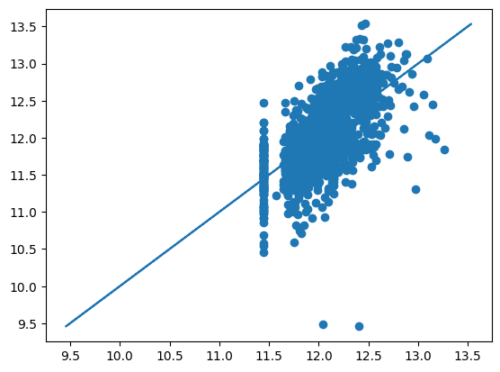

You are likely to see that the R2 score from our gradient descent method (the most common ML algorithm) is not the same, and perhaps a bit worse, from your results using scikit-learn LinearRegression. Again, this is likely due to ‘hidden’ operations inside that packages that I have not yet been able to reverse engineer. Appart from the bias and feature rescaling, LinearRegression might have some clever ways to, e.g., deal with major outliers in the measurements.

Still, by playing around with different combinations of features for about half an hour, I myself was able to get R2 scores from LinearRegression of almost 0.9 and around 0.85 from our own gradient descent method above. Not bad for just a simple linear regression model!

Reminder: if you just read through this notebook without changing much, you’re not done yet ;) ! In this early-ish lab, I gave you all/most of the skeleton code you’ll need, but the objective of this lab is for you to now experiment with different subsets of features, potentially engineering some non-trivial features, and trying out for yourself how to construct the best ML multivariate linear regression model to best predict housing prices from the dataset that you were provided with in the very top. The key variable is the accuracy (e.g. in terms of R2) of your predictions on validation data that were not used in the model training (fit). This is a measure of how well you can expect your model to work to predict for future houses for which true sale prices are not know.

Summary & Next Steps

This lab was a classical ML example of using multivariate but all-linear numeric regression. A separate lab for this week considers multivariate and non-linear regression for an actual Earth Sciences problem.

Once you’ve mastered these labs and the ideas behind them, you’ll already have the Machine Learning tools to analyze data for a wide range of Science and Engineering problems where the thing you want to predict is a continuous variable.

Next week, you’ll learn how we can readily generalize these ideas even further to predict things where your target variable can only take on discrete values. For example, whether a pixel in a satellite image is water/land/grass/forest etc, which we can label as classes 1, 2, … , nr_classes. Those schemes are called logistic regression.