Which platform should I choose?

📖 Review the Lecture notes

Lab 1 – Linear Regression

In this first introductory lab, you will explore your first ‘machine learning’ algorithm: a linear numerical regression in terms of a single variable. The goal is to start familiarizing yourself with coding python in a jupyter notebook.

For this reason, I will not throw you in at the deep end and ask you to code the full regression model from scratch (which is provided in the lecture notes jupyter notebook). Instead, you will use the convenient pre-coded algorithms available in the excellent Machine Learning library scikit-learn. We will use many other routines from that library in future labs.

In addition, all labs will use the numpy library, which contains much of the algebra functionality that you would find in, e.g., Matlab, and the matplotlib library, which gives you much of the same visualization options from Matlab (though a bit more limited).

Finally, we will work with some real data that we will pull in directly from a scientific journal. The particular data are provided as an Excel file. Python’s main package to work with spreadsheet data, which can contain a mix of numerical values and rows/columns of text (strings), is pandas. A spreadsheet read into panda is called a dataframe.

To summarize, this lab will be a first introduction to the following python packages:

• numpy
• matplotlib
• pandas
• scikit-learn

Suggestion: double click on the above (or any other) text cell to see how you can format text in jupyter notebooks, i.e. option to change fonts to bold/italic, indicate text as code snippets, or create different section headers by starting text with one or more hash # symbols. Below you can also see some formatted equations, using LaTeX notation.

Before we get to the linear regression, I will provide some introductory examples and exercises for those of you who have never used python (and/or matlab) before. If you are familiar with those concepts, by all means skip ahead.

Load packages

In general, I would suggest loading all python packages that you want to use in a single code cell in the very top of a jupyter notebook. At least that’s my personal preference to easily have this all on one place and see which packages I have/haven’t loaded. In this first lab, though, I will load packages as they are needed to explain what they are along the way.

Let’s start by loading the 4 main packages mentioned above:

import numpy as np
import matplotlib.pyplot as plt
import pandas as pd

Each of these statements imports an entire module (numpy, matplotlib, pandas) and assigns a prefix that you will use to tell python when you want to use a function from a specific module. This is because multiple modules may contain functions with the same name, which may each function somewhat differently.

Numpy and Matplotlib

Let’s start with some simple examples. Both in Matlab and in python’s numpy, you can generate a list (vector/rank-1 array) of numbers between some minimum xmin and some maximum xmax in n steps by the linspace function, which in numpy you would prefix with np.linspace.

Without knowing all the functions and variables in numpy, you can usually guess. For example, if you want to use the number \(\pi\) (see how I format this in this text box by double clicking on it), you just use np.pi.

Basic plotting works the same as in Matlab, but now we prefix those function names with plt for the matplotlib library.

# define minimum and maximum
# Note that I put this here primarily to show how lines that start with a
# hash symbol are not executed as python code, i.e. this is how you can add comments
# to make your code more readable.
# This is particularly important when you write python code outside of jupyter,
# in which case you won't have the convenient mixing of code and text cells.
xmin = 0
xmax = 4*np.pi
n = 100
x = np.linspace(xmin,xmax,n);
y = np.sin(x);

plt.plot(x,y);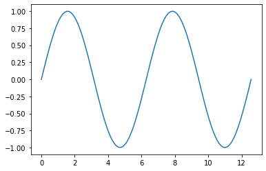

Excercise: Spend some time playing with the above code cell: try a few other functions (cosine, exponent, square-root, log). Can you figure out how to plot more than one function in the same figure?

Now let’s prettify this into a proper scientific type figure, which needs axes lables, a title, perhaps a legend. You can also change line colors, thickness, use lines and/or symbols, all pretty much the same as in Matlab. You’ll have plenty of opportunity to play around with all these options throughout the semester. Here’s some links that summarize different markers and linestyles, with other matplotlib options you can select in the menu on the left (a simple google search will also give you many other websites on the topic).

x = np.linspace(0,6*np.pi,100);
plt.plot(x,np.sin(x), 'rd-', label='sin(x)');
plt.plot(x,np.cos(x), 'bx-', label='cos(x)');

plt.title('Plot of functions')
plt.xlabel('Independent variable $x$')
plt.ylabel('Dependent variable $y$')

plt.legend(loc='lower left');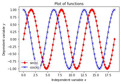

Working with arrays

One of the most important things in working with Matlab or python’s numpy is to work with certain subsets (slices) of data that are organized in arrays (vectors, matrices, or multidimensional arrays). In this sections I will provide a somewhat comprehensive set of examples to illustrate (and for your to practice with) how this works.

Here is an example where I only plot a few subsets of our variables \(x\) and \(y\). See if you understand what the code below does. This example also shows you a few other things, such as using multiple subplots, and two different ways of plotting multiple curves in a single plot.

xmin = 0
xmax = 4*np.pi
n = 100
x = np.linspace(xmin,xmax,n);
y = np.sin(x);
y2 = np.cos(x);

plt.figure(figsize=[12,6])
# Subplots: make a single row with two columns of plots, and generate the first
# of those two plots:
plt.subplot(1,2,1)
plt.plot(x[0:20],y[0:20],'r', x[35:55],y[35:55],'gx', x[70:-5],y[70:-5],'b');

# Now make a second plot.
# By comparing this plot to the first panel, you can see that you can either
# add multiple curves in the same plotting command, or add them separately,
# which perhaps is more readable.
plt.subplot(1,2,2)
plt.plot(x[0:20],y2[0:20],'r')
plt.plot(x[35:55],y2[35:55],'gx')
plt.plot(x[70:-5],y2[70:-5],'b');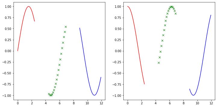

To expand a little, look at a simpler example. Let’s create a 1-dimensional array (called rank-1) with numbers 1, …, 10. By default, linspace creates floating numbers, but for cleaner outputs I convert those to integers by using the numpy code .astype(int).

x = np.linspace(1,10,10).astype(int)
x

array([ 1,  2,  3,  4,  5,  6,  7,  8,  9, 10])

If we want to use (slice) the first 5 and last 5 numbers, we can use:

first5 = x[0:5]
last5  = x[5:10]

print("First five numbers:", first5, 'and last five numbers:', last5)

First five numbers: [1 2 3 4 5] and last five numbers: [ 6  7  8  9 10]

A big difference between python and matlab is that python counts from zero while matlab counts from 1 as the first element in an array. For the same reason, when you specify a range of indices, the ending index itself is actually not included. In other words, you might think that x[0:5] would be 6 values (x[0], x[1], x[2], x[3], x[4], x[5]), but that last element, x[5], is not included. For the same reason, because counting starts at 0, x[5] is actually the 6th element.

Warning: this counting is confusing and a major source of coding errors. Whenever in doubt, it is always a good idea to plug in another code cell and try things out with a simple example. A useful way to check it with numpy’s shape function:

np.shape(x)

(10,)

np.shape(x[0:5])

(5,)

note that you don’t have to specify 0 as the starting element, because that is the default, so you can also use shorter notation:

np.shape(x[:5])

(5,)

and similar for the last element:

np.shape(x[5:])

(5,)

If you don’t know the size/length of the array, you can also specify a range until, say, 4 elements from the end as

x[:-4]

array([1, 2, 3, 4, 5, 6])

All the examples above are for a rank-1 array, a vector or simple list of numbers. Of course quite often we will work with rank-2 arrays (whether algebraic matrices or sets of numbers derived from spreadsheet-like data).

To give you an example, we can reshape the above 10-element vector in a matrix with 2 rows and 5 columns by using the same command as you could use in Matlab:

x2 = np.reshape(x,[2,5])
x2

array([[ 1,  2,  3,  4,  5],
       [ 6,  7,  8,  9, 10]])

You could also create a small array like this by explictly typing out the element values:

test = np.array([[1,2,3,4,5],[6,7,8,9,10]])
test

array([[ 1,  2,  3,  4,  5],
       [ 6,  7,  8,  9, 10]])

Note in the above that there are two outer brackets to indicate that this is a 2-dimensional (rank-2) array. Within the outer brackets, we can specify the individual rows in single brackets. This is similar to how you would do this in Matlab or Mathematica. Here’s another example:

test = np.array([[1,2],[3,4],[5,6],[7,8],[9,10]])
test

array([[ 1,  2],
       [ 3,  4],
       [ 5,  6],
       [ 7,  8],
       [ 9, 10]])

As always, it can be useful to check the shape of arrays:

# add code to check the shape of the above arrays

Exercise: define a variable that gives you this array

\(x_3 = \left( \begin{array}{cc} 2 & 3 & 4 \\ 7 & 8 & 9\end{array}\right)\)

by using index notation. In other words, subset this array with index ranges from the x2 array defined above.

# add code to create the above matrix by specifying row and column index ranges out of the x2 array.

Adding/subtracting/multiplying arrays

It is easy to add and subtract arrays, and this can be done either using simple notation like:

double_x = x + x
double_x

array([ 2,  4,  6,  8, 10, 12, 14, 16, 18, 20])

x - double_x

array([ -1,  -2,  -3,  -4,  -5,  -6,  -7,  -8,  -9, -10])

and the same for a higher rank array:

x2 + x2

array([[ 2,  4,  6,  8, 10],
       [12, 14, 16, 18, 20]])

or with more explicit numpy functions:

np.add(x,x)

array([ 2,  4,  6,  8, 10, 12, 14, 16, 18, 20])

np.subtract(x,x)

array([0, 0, 0, 0, 0, 0, 0, 0, 0, 0])

Things get a bit more subtle when we want to multiply, divide, or exponentiate arrays. In both matlab and python there are two ways of doing this. The first simply treats an array as a set of numbers and multiplies/divides/exponentiates element-by-element:

x * x

array([  1,   4,   9,  16,  25,  36,  49,  64,  81, 100])

x**2

array([  1,   4,   9,  16,  25,  36,  49,  64,  81, 100])

np.multiply(x,x)

array([  1,   4,   9,  16,  25,  36,  49,  64,  81, 100])

np.divide(x,x)

array([1., 1., 1., 1., 1., 1., 1., 1., 1., 1.])

np.multiply(x2,x2)

array([[  1,   4,   9,  16,  25],
       [ 36,  49,  64,  81, 100]])

etc. Note that these are not algebraic operations on vectors/matrices. If you remember your algebra, the ‘product’ of 2 vectors, or rather the inner product or dot product, reduces the rank and gives you a single number (in the case of multiplying a vector with itself, this is the length of that vector, which itself is a directional ‘arrow’). You should also remember that you can only take dot products between row and column vectors. Similarly, the algebraic product of, say, a \(3\times 4\) array and a \(4\times 8\) array will be a \(3\times 8\) array (and those inner dimensions, 4 in this case, have to match).

For vectors, 2 ways of computing the dot product are:

x.dot(x)

385

np.dot(x,x)

385

and for matrices:

# uncomment the line below and see what happens:
# np.matmul(x2,x2)

Why does the above give you an error?

Exercise: fix the above error by using numpy’s transpose function np.transpose. Check as always with np.shape the shape of the x2 array before and after transposing. You can do everything in one line or define a separate variable for the transpose of x2.

What is the shape of the matrix product of these two arrays?

# add code to compute matrix product and print the size of the resulting output/variable.

Note, you can also use the ampersand symbol @ as a shorter notation to take the proper matrix product of two arrays with suitable dimensions.

Exercise: you can never have enough practice with this. Spend a little time making different arrays of different sizes, defining new arrays as subsets of those, and performing algebraic operations either in the element-by-element sense or in the vector-matrix sense.

To be very clear: adding or subtracting matrices in proper algebra is already the same as adding/subtracting the individual elements of each array, so there is no complication there.

It is often convenient to assign a variable name to an array of certain dimensions and set all elements initially to 0 or 1 (or perhaps increasing integers, as above). This way you know the array has the correct dimensions, and the ‘computer’ knows it too and already assigns the right amount of computer memory (RAM). Then you can fill in the elements one-by-one in a loop, or through index subsetting later. Here are some examples:

arr_1 = np.zeros([4,7])
arr_1

array([[0., 0., 0., 0., 0., 0., 0.],
       [0., 0., 0., 0., 0., 0., 0.],
       [0., 0., 0., 0., 0., 0., 0.],
       [0., 0., 0., 0., 0., 0., 0.]])

arr_2 = np.ones([4,7])
arr_2

array([[1., 1., 1., 1., 1., 1., 1.],
       [1., 1., 1., 1., 1., 1., 1.],
       [1., 1., 1., 1., 1., 1., 1.],
       [1., 1., 1., 1., 1., 1., 1.]])

# the identify matrix, which is zero everywhere except one on the main diagonal
arr_3 = np.eye(4)
arr_3

array([[1., 0., 0., 0.],
       [0., 1., 0., 0.],
       [0., 0., 1., 0.],
       [0., 0., 0., 1.]])

Now let’s change some of the ‘ones’ in array arr_2 by inserting values from our earlier array x2. First, we’ll remind ourself of the size of the latter array:

np.shape(x2)

(2, 5)

And here’s an example that illustrates a bunch of index wizzardry. We take all the rows of x2 but only the first 4 columns (x2[:,:-1], which is the same as x2[:,:4] in this case, because there are 5 columns). Then we insert these values into the first 2 rows and 2nd to 6th columns of arr_2 as follows:

arr_2[0:2,2:6] = x2[:,:-1]
arr_2

array([[1., 1., 1., 2., 3., 4., 1.],
       [1., 1., 6., 7., 8., 9., 1.],
       [1., 1., 1., 1., 1., 1., 1.],
       [1., 1., 1., 1., 1., 1., 1.]])

again, it is easy to make mistakes in these index ranges and getting the numbers to show up where you wanted them.

Exercise: Play arround with this example a little and see if you can assign some subset of the x2 array into, say, the top-left, bottom-right, or wherever, regions of the larger zero-matrix arr_1.

Warning: when you try a couple of different substitutions you may get suprising results, because each of those already modified the original arrays arr_1 or arr_2. You’ll probably want to redefine, say arr_1 = np.zeros([4,7]) at the start of this code cell before you make changes.

# experiment with array substitutions

One more important subtlety that is different in python/numpy as compared to matlab. If you paid attention above when I showed how to take dot-products of vectors, you may (?) have wondered why we didn’t have to make a distinction between row and column vectors. To repeat the example, and pay attention again to the vector shape:

a = np.linspace(1,5,5).astype(int)

print("Shape of vector a", np.shape(a))

print("Dot product of vector a with itself", a.dot(a))

Shape of vector a (5,)
Dot product of vector a with itself 55

so you can see that this vector \(a\) only has one dimension, and in python/numpy you can do vector products between such 1-dimensional arrays without having to take transposes, i.e. without distinguishing row from column vectors. For some/many applications, such as almost all machine learning routines in scikit-learn, we have to be specific on whether a vector is a row or column vector. For a row vector, we have 1 row and as many columns as the length of that vector, say n, and for a column vector we have to specifically say that it only has one column with n rows.

There are different ways of doing this. Below I show examples of specifying \(a\) as either a row or column vector by either explicitly defining the range of the two dimensions (one of which is 1), or by using the python notation ‘None’, which just adds a dimension along the first or second axis/dimension. Both approaches give the same result. In both cases, we define a rank-2 array (in other words a matrix), but either with just 1 row or just 1 column. Pay attention to the np.shape of each result.

b = np.zeros([1,5]).astype(int)
b[0,:] = a

c = np.zeros([5,1]).astype(int)
c[:,0] = a

d = a[None,:]
e = a[:,None]

print("Shape of matrices a:",np.shape(a), ", b:", np.shape(b) , ", c:", np.shape(c), ", d:", np.shape(d), ", and e:", np.shape(e))

Shape of matrices a: (5,) , b: (1, 5) , c: (5, 1) , d: (1, 5) , and e: (5, 1)

Note that \(b\), \(c\), \(d\), \(e\), are now defined as rank-2 arrays, so if we want to select (or slice) certain (ranges of) elements, we have to specify those index ranges in both dimensions, one of which only has 1 value:

b[0,2:4]

array([3, 4])

c[2:4,0]

array([3, 4])

Now, when we take the dot product of two 1-dimensional arrays we get a single scalar number:

a.dot(a)

55

Using matrix multiplication (using the shorthand @ notation) we get the same result:

a @ a

55

and the result is an empty array (it is a scalar, not an array):

np.shape(a @ a)

()

When we define the same numbers as rank-2, i.e. 2-dimensional, arrays, we have to be careful with the order. If we multiple a \(1\times 5\) vector with a \(5\times 1\) vector (row vector times column vector), we get the same single number, but it you pay attention to the notation in the output, this is still a rank-2 array/matrix. It just only has 1 row and 1 column:

d @ c

array([[55]])

np.shape(d @ c)

(1, 1)

But if we change the order and thus multiple a \(5\times 1\) vector with a \(1\times 5\) vector (column vector times row vector), we get a \(5\times 5\) array.

[In algebra terms, matrix multiplication is not commutative, and contracts on the middle index.]

c @ d

array([[ 1,  2,  3,  4,  5],
       [ 2,  4,  6,  8, 10],
       [ 3,  6,  9, 12, 15],
       [ 4,  8, 12, 16, 20],
       [ 5, 10, 15, 20, 25]])

btw, this also works when using dot notation:

c.dot(b)

array([[ 1,  2,  3,  4,  5],
       [ 2,  4,  6,  8, 10],
       [ 3,  6,  9, 12, 15],
       [ 4,  8, 12, 16, 20],
       [ 5, 10, 15, 20, 25]])

b.dot(c)

array([[55]])

I fully appreciate that all the above array manipulations are tedious and at this point perhaps a bit confusing. It is to be expected that these examples will not immediatetly sink in nor make you ‘fluent’ in these types of operations.

My goal with this section is to give you a little bit of initial practice and a ‘reference guide’ that you can return to throughout this course when you get stuck while working on more interesting problems, such as the first real problem below, in which you will implement a linear regression model, which will already use a number of these notations.

Linear regression with scikit-learn

Scientific problem statement

In this lab, we will work with real published scientific field data, collected by one of our own Earth Sciences (former) students, Devin Smith (et al.).

Without going into much detail, this paper explores Local Meteoric Water Lines (LMWL), which can be compared to Global Meteoric Water Lines (GMWL). These lines refer to a linear correlation between the isotopes Oxygen-18 (\(\delta^{18}\)O) and Deuterium (\(\delta^2\)H), which is cause by a fractionation between evaporation from oceans and precipitation. If you’re interested, you can read the wikipedia page.

The GMWL has been shown to follow the linear relationship:

\(\delta^2\)H $ = 8^{18}$O \(+ 10\).

Local deviations from this relationship, i.e. as shown in LMWL, are a way to track regional precipitation trends/events (in other words, differences from the global average precipitation as compared to evaporation from oceans). This is done by taking field measurements over time of these isotope ratios from water samples collected from, e.g., rivers/streams/lakes.

I encourage you to have a look at the actual paper by Devin Smith et al.: Local meteoric water lines describe extratropical precipitation

As good scientific practice, this paper includes Supporting Information that includes all the raw data. The data is organized in an Excel file, and fortunately, the journal Hydrological Processes, published by Wiley, provides a direct link/url to those data, which we can suck directly into this jupyter notebook, without having to download to your local computer and/or upload into the google cloud.

Still, you should download the file and open it in Excel so you can see all the data in a format/software that is perhaps more familiar. This may make it easier to understand the somewhat more complicated initial steps to load these data into a pandas dataframe in python.

Loading measurements into pandas dataframe

For cleaner code, it can be helpful to define a string variable that holds the (long) URL pointing to these data:

file_url = 'https://www.hydroshare.org/resource/769780f3dd9d444b8bb9e0560fa292de/data/contents/Central_Ohio_Precipitation_Isotopic_Composition_2012_2018_HydroShare.xlsx'

Next, to open/stream/import a file directly from a URL, we need another python module. There are probably several modules that can do this, but I’m using the ‘requests’ module here (again, in general I would suggest combining all these module import in one code cell in the top of a jupyter notebook):

import requests

The code below loads the file from a URL into a ‘fake’ excel file that only lives in memory (i.e. it won’t actually be stored as a temp.xls file anywhere):

r = requests.get(file_url);
open('temp.xls', 'wb').write(r.content);

The next code reads the excel file into a pandas dataframe. If you google anything on dataframes, you will see that the convention is to use df as the variable name for a dataframe, so I will follow that convention. But just like any other variable you can choose whatever name you like.

Note that when reading in the excel file, I skip the first 3 rows of that file because it contains a bunch of header information that we don’t need. Also, those rows in the excel file are formatted with a different number of columns than the rest of the data, which would cause all kinds of headaches in the resulting dataframe.

df = pd.read_excel('temp.xls',skiprows=3)

Whenever you read in or define a dataframe, it is useful to print the ‘head’ of it, which is simply the first few rows and shows you the names assigned to rows and columns:

df.head()

	Location	Sample ID	Date	Time	Precipitation	δ18O [‰]	δ2H [‰]	d-excess [‰]	Precip [cm]	Avg Air Temp [°C]	Average Relative Humidity [%]	Average Wind Speed [km/h]	Wind Direction [360°]
0	MSFLD	MSFLD12-01	2012-10-18 00:00:00	NaN	R	-9.536605	-67.917983	8.374861	0.13	13.7	70.0	2.6	215.683681
1	MSFLD	MSFLD12-02	2012-10-19 00:00:00	NaN	R	-15.225769	-112.409574	9.396580	0.36	10.7	74.0	2.3	202.917708
2	MSFLD	MSFLD12-03	2012-10-26 00:00:00	NaN	R	-9.119374	-52.921759	20.033237	0.38	12.4	81.0	2.6	116.794556
3	MSFLD	MSFLD12-04	2012-10-27 00:00:00	NaN	R	-12.930548	-84.575077	18.869310	1.45	7.9	93.0	3.5	20.497257
4	MSFLD	MSFLD12-05 (SANDY)	2012-10-28 00:00:00	NaN	R	-13.255571	-86.329866	19.714701	1.85	5.9	90.0	4.5	21.851177

This output also demonstrates why we have to use a pandas dataframe at all. We really just want to work with a (numpy) array of numerical values, but this excel file has several columns (e.g., the Sample ID, Precipitation Location, Time, Date) that are strings or in this case formatted dates. Numpy arrays only allow numerical values, while pandas dataframes allow for various other data types, such as strings. In this course, and in machine learning / data analytics more generally, dataframes are mostly used as an intermediate step to extract the numerical values (rows/columns) of interest and then often turn those into numpy arrays.

This is how you can just see all the column names/headers in the dataframe:

print("Column headers", df.columns[1:])

Column headers Index(['Sample ID ', 'Date ', 'Time', 'Precipitation ', ' δ18O [‰]',
       ' δ2H [‰]', 'd-excess [‰]', 'Precip [cm]', 'Avg Air Temp [°C]',
       'Average Relative Humidity [%]', 'Average Wind Speed [km/h]',
       'Wind Direction [360°]'],
      dtype='object')

For the purpose of this lab, we are only interested in the columns for the \(\delta^2\)H and \(\delta^{18}\)O isotope values:

col_select = df.columns[5:7]
print("Column headers of interest:" , col_select)

Column headers of interest: Index([' δ18O [‰]', ' δ2H [‰]'], dtype='object')

I won’t go into a lot of details on working with pandas dataframes here, and go straight to just extracting the data we need. When working with dataframes, you can extract rows and/or columns (partially or all of them) by specifying the numeric values of the rows, which you can see on the left column, and the (string) names of columns, which you see in the top:

df[col_select]

	δ18O [‰]	δ2H [‰]
0	-9.536605	-67.917983
1	-15.225769	-112.409574
2	-9.119374	-52.921759
3	-12.930548	-84.575077
4	-13.255571	-86.329866
...	...	...
493	-20.336793	-148.063014
494	-14.721997	-102.415207
495	-13.782884	-98.165926
496	-16.951857	-125.201807
497	-5.210582	-24.658753

498 rows × 2 columns

Or if you were to spell it out explicitly, here is an example of just selecting one column:

df[' δ18O [‰]']

0      -9.536605
1     -15.225769
2      -9.119374
3     -12.930548
4     -13.255571
         ...    
493   -20.336793
494   -14.721997
495   -13.782884
496   -16.951857
497    -5.210582
Name:  δ18O [‰], Length: 498, dtype: float64

Note that you have to be careful that all the spaces etc are exactly correct, so it is easy to make mistakes (see below). This is of course especially the case when you use someone else’s data.

# uncomment below and execute
# df['δ18O [‰]']

This is why it is easier safer to just specify that you’re interested in, say, the 5th column, i.e. as:

df[df.columns[5]]

0      -9.536605
1     -15.225769
2      -9.119374
3     -12.930548
4     -13.255571
         ...    
493   -20.336793
494   -14.721997
495   -13.782884
496   -16.951857
497    -5.210582
Name:  δ18O [‰], Length: 498, dtype: float64

Converting data to numpy array

So now for the important step: we again just extract the 2 columns of interest, and simply by adding .to_numpy(), we transform these data to a numpy array. For convenience, we assign this numpy array the variable name isotope_data.

isotope_data = df[col_select].to_numpy()

The linear regression model, which we’re about to get to, is going to correlate the \(\delta^{18}\)O isotope abundances to those of \(\delta^2\)H. For this purpose it is useful to treat the latter as the independent variable, or ‘feature’ \(x\) and the former as the dependent variable or ‘target’ \(y\) (in machine learning parlance).

# Features:
x = isotope_data[:,0];
# Target:
y = isotope_data[:,1];

Exercise: make a nice plot of \(\delta^{18}\)O versus \(\delta^2\)H isotope abundances.

# add a plot here of y versus x and add appropriate axes labels and title

You should visually see that the relation between these isotope abundanes is linear, but obviously with some experimental/measurements noise.

Our goal is to fit a linear curve to these data. Or more specifically, to find the linear model $^2 $H $= _0 + _1^{18} $O with values for the intercept \(\theta_0\) and slope \(\theta_1\) with the smallest fitting error (as defined by a least-squared-error, absolute error, or R2 value).

Splitting into training and validation data

We could easily just fit a linear model to all the isotope data directly, but for this ‘machine learning’ (ML) exercise, we will use the standard ML approach of splitting the data into ‘training’ and ‘validation’ data.

To explain the basic reasoning for this, consider this ‘thought experiment’ for an extreme example: if we only had 2 measurements, there is only one linear curve that fits both those points and it would have 100% accuracy (there is only one straight line that connects two points). However, if we made one more measurement, and all measurements have some error, that point would be extremely unlikely to fall on the exact same straight line. So the initial fit to 2 points would likely not be the best fit for all 3 points and indeed have a large fitting error. Basically, that first model was overfitted.

To generalize: if we have 100 measurements, a robust way to fit a model to those measurements is to find the intercept and slope that most accurately fits those 80 points, i.e. gives the lowest fitting error. But then the important next step is to see how well that same model fits the other 20 points that were not part of the initial fitting (regression). If the fitting error is still more or less the same, the model is (more) robust. This is why these are called the validation data.

A subtlety that we’ll deal with later is that if all the data were ordered from small to large numbers, it wouldn’t work well to take the first 80% of training and the last 20% for validation. A better way is to first shuffle the data into a random order. Fortunately, it turns out that these measurements are already ‘shuffled’ (because precipitation events occur somewhat randomly at different times).

Let’s take the first 80% of data for training and the other 20% as validation data.

nr_data_points = len(x)

splitat = int(0.8*nr_data_points)
print("Total number of data points", nr_data_points, 'split into ',splitat ,'training data and ',nr_data_points - splitat , 'validation data.' )

Total number of data points 498 split into  398 training data and  100 validation data.

See below how we can define 2 arrays at once with each of the code lines, and how we use ‘None’ to define rank-2 arrays with just one column. This is required when using scikit-learn’s linear regression model later.

# train, validation set split
x_trn, x_val = x[:splitat,None], x[splitat:,None]
y_trn, y_val = y[:splitat,None], y[splitat:,None]

always good to check array dimensions:

np.shape(y_trn)

(398, 1)

Visualize data

Here’s a different kind of plot, a scatter plot, to visualize noisy data that don’t fall on a neat curve. We separately plot the training and validation data, and Matplotlib will automatically use different colors for each. This way you can see that indeed the data were already shuffled and the validation data show good overlap with the training data.

plt.scatter(x_trn,y_trn)
plt.scatter(x_val,y_val);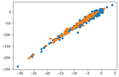

Exercise: Make a plt.plot lineplot of the same data to see why this is not a good option here.

# add line plot of training and/or validation data

Scikit-learn linear regression

Load the scikit-learn LinearRegression model:

from sklearn.linear_model import LinearRegression

Note that we’re doing this a bit different from how we loaded numpy and pandas. When we use syntax like

import numpy as np

we import the entire module numpy and every time we want to use a specific function from that module, we have to prefix it with .np (e.g., np.sin). In the above example for the linear regression, we only import a single specific function from that module and we can then use that name directly without a prefix.

The entire regression can now be done with just a single line of code:

linear_regression_model = LinearRegression().fit(x_trn, y_trn)

The notation of how these things are done in Python is a bit confusing as compared to how, e.g., Matlab or languages like Fortran/C work. At this stage, it may be easiest to just google/copy/paste examples and see how they work.

As you may guess from the above notation, LinearRegression() fits a linear model to predict ‘targets’ y_trn from ‘features’ x_trn, based on our training data. Note that the google colab version of jupyter, which we are working in, has some other very useful features that are not standard in jupyter. For example, when you hover over a function, such as LinearRegression, you will see a pop-up that tells you what this function does and how it works (input/output etc). You can click on the links within the pop-up for more info.

Exercise: hover over LinearRegression to see this pop-up window and click on ‘open in tab’ which will open all the info in a frame on the right of this window. You can see an example similar to the above of fitting a \(y\) to an \(X\) array of data, and below you can see how you can get the fitting score (accuracy) of the fit and the linear fitting coefficient (slope) and intercept. Finally, the information shows how to then use this model to make predictions.

Another useful way to explore a weird variable like the above linear_regression_model is to use python’s dir function:

dir(linear_regression_model)

['__abstractmethods__',
 '__class__',
 '__delattr__',
 '__dict__',
 '__dir__',
 '__doc__',
 '__eq__',
 '__format__',
 '__ge__',
 '__getattribute__',
 '__getstate__',
 '__gt__',
 '__hash__',
 '__init__',
 '__init_subclass__',
 '__le__',
 '__lt__',
 '__module__',
 '__ne__',
 '__new__',
 '__reduce__',
 '__reduce_ex__',
 '__repr__',
 '__setattr__',
 '__setstate__',
 '__sizeof__',
 '__str__',
 '__subclasshook__',
 '__weakref__',
 '_abc_impl',
 '_check_feature_names',
 '_check_n_features',
 '_decision_function',
 '_estimator_type',
 '_get_param_names',
 '_get_tags',
 '_more_tags',
 '_preprocess_data',
 '_repr_html_',
 '_repr_html_inner',
 '_repr_mimebundle_',
 '_residues',
 '_set_intercept',
 '_validate_data',
 'coef_',
 'copy_X',
 'fit',
 'fit_intercept',
 'get_params',
 'intercept_',
 'n_features_in_',
 'n_jobs',
 'normalize',
 'positive',
 'predict',
 'rank_',
 'score',
 'set_params',
 'singular_']

This shows a whole bunch of attributes. If you scroll through them, you’ll see the ones that we’re interested in: coef_, intercept_ ,and score. The first of those are just output variables, while the last one is actually like a function. Let’s explore:

r2_score = linear_regression_model.score(x_trn,y_trn)
r2_score

0.9728780147520028

Again, you can now hover just over .score to see how it works. The help info shows (either in the pop-up or you can expand again into a full window) that to get this score you have to provide \(x\) and \(y\) inputs, and the output is a R2 score. In this case, we get an R2 on our fit to the training data of 0.97, which is very good indeed.

Now let’s assign some variable names to the slope and intercept that we found in the above linear regression fit (again, you can hover over .coef_ etc to get info):

slope = linear_regression_model.coef_
intercept = linear_regression_model.intercept_

print("Fitting coefficients are slope:", np.round(slope,3), 'and intercept', np.round(intercept,2) )
print("Precision of our fit to training data, as measured by R2 score, is:", np.round(r2_score,2))

Fitting coefficients are slope: [[7.699]] and intercept [8.37]
Precision of our fit to training data, as measured by R2 score, is: 0.97

In other words, we find a $^2 $H $= 7.7 ^{18} $O \(+ 8.8\), pretty close to the relation $^2 $H $= 7.58 ^{18} $O \(+9.16\) in the paper (also with R2 $ = 0.97$). The difference is probably because in the paper all data were fitted at once, whereas we only fitted to 80% of those data as a training set (more on that below).

Quick aside: from the square brackets, you can see that the slope is given as a (1,1) rank-2 array while the intercept is given as a (1,) rank-1 one-dimensional array/vector. This is because linear regression can also be applied to many variables (next lab), in which case there are multiple slopes and intercepts. Also note how I used np.round to round results to 2 digits when I output these results as text. Try removing the rounding functions to see what the print statement would have looked like otherwise.

Now that we have the fitting results, which in this case are simply the intercept and slope, we can use this model to make predictions for new data. In our case, we set asside a set of independent validation data that were not seen when we fitted our training data. We can make those predictions in two ways.

First, we can use the .predict() function that is part of the scikit-learn LinearRegression model:

pred_1 = linear_regression_model.predict(x_val)
pred_1

array([[ -48.98108353],
       [-111.41178008],
       [ -28.63465335],
       [-123.5327714 ],
       [-136.2379995 ],
       [-185.62906926],
       [-198.85127004],
       [ -94.46921607],
       [ -34.29106371],
       [ -88.5646215 ],
       [-193.6994775 ],
       [ -30.22047483],
       [ -34.34078172],
       [ -89.56790568],
       [ -43.5472776 ],
       [ -93.44054325],
       [ -95.11439691],
       [-102.49810656],
       [ -86.08077429],
       [ -49.17509749],
       [-128.74258326],
       [ -20.37311634],
       [ -47.64525838],
       [ -34.58138778],
       [ -34.64725257],
       [ -32.50870498],
       [ -67.4280744 ],
       [ -45.68144715],
       [ -54.67388737],
       [ -88.90656061],
       [-120.54914681],
       [ -37.49164391],
       [ -15.33940919],
       [-119.0133033 ],
       [ -21.35100873],
       [ -72.55965739],
       [  16.63881262],
       [  -9.6689337 ],
       [ -11.90368031],
       [ -33.7277221 ],
       [ -45.02533529],
       [ -62.43596407],
       [ -40.86346957],
       [ -49.72660877],
       [ -48.33237908],
       [ -28.39828534],
       [ -40.69303757],
       [ -48.78767475],
       [ -14.18218967],
       [ -36.48510105],
       [ -35.54582074],
       [ -38.88526204],
       [ -44.52171428],
       [ -70.64125413],
       [ -37.73228693],
       [ -26.63495986],
       [ -14.67484333],
       [  -1.00489191],
       [  -6.9404251 ],
       [ -28.12641081],
       [ -13.97714191],
       [ -63.9714726 ],
       [ -69.32635117],
       [ -69.89365114],
       [ -57.5618367 ],
       [ -57.42417516],
       [ -10.48666732],
       [ -53.74900959],
       [ -19.74635414],
       [ -26.28673883],
       [ -53.47510661],
       [ -42.43851767],
       [ -34.18522282],
       [ -15.91837702],
       [ -28.73350184],
       [ -67.46512133],
       [ -41.18146835],
       [ -15.73993602],
       [ -96.44514184],
       [-109.28932394],
       [ -91.56522785],
       [ -32.08305879],
       [ -59.17134947],
       [ -39.46234404],
       [ -76.18878244],
       [-127.06458529],
       [ -88.04452968],
       [-124.74813788],
       [ -92.16658792],
       [ -87.94432712],
       [ -95.46824347],
       [ -62.50451876],
       [ -95.96653461],
       [ -88.52978614],
       [-105.32599721],
       [-148.21133188],
       [-104.98115464],
       [ -97.75061168],
       [-122.14958836],
       [ -31.74962033]])

What this does is for each input value x_val, which are measured values of \(\delta^{18}\)O, the prediction gives a value for \(\delta^2\)H using the formula above: $^2 $H $= 7.7 ^{18} $O \(+ 8.8\).

It never hurts to check the shapes of these arrays:

print("Shapes of validation inputs and predicted outputs", np.shape(x_val), np.shape(pred_1))

Shapes of validation inputs and predicted outputs (100, 1) (100, 1)

Note that the whole point of doing this is that we also have actual measured values for \(\delta^2\)H, so we can compare predictions to actual measurements. First, let’s do this visually:

plt.plot(x_val, pred_1,'r-')
plt.scatter(x_val, y_val);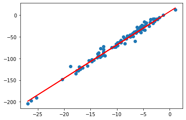

To see how well this model fits the independent validation data, I’ll illustrate how to get the accuracy in a different way. Similar to how we loaded the LinearRegression model itself as a single function pulled out of sklearn, we can import a number error/accuracy metrics. I’ll import a couple of those at once, and you can try out different options.

from sklearn.metrics import mean_absolute_error,mean_squared_error,r2_score

Here is how to get the accuracy of the fit in the above plot.

r2_val = round(r2_score(pred_1, y_val ),2)
print("RMS error on validation data is", r2_val)

RMS error on validation data is 0.98

Interestingly, and a bit unusually, the fitting accuracy on the validation data is actually even slightly higher than on the training data. This means that our model is pretty good and can be generalized to new measurements.

[Though, as wel will discuss in future lectures/labs, this is largely because these validation data still fall within the same range, i.e. within the minimum and maximum values of the training data.]

As mentioned a few cells earlier, we can also do the prediction in a different way without using the prediction function of LinearRegression. Specifically, we can use enter the linear function directly as applied to our validation input data x_val:

pred_2 = intercept + slope * x_val

This gives exactly the same result.

Exercise: check this by taking the difference between pred_1 and pred_2. This will give a vector of 100 numbers (the length of x_val, pred_1 and pred_2), so I would suggest summing the result (np.sum) to get a sum of those differences, which should still be zero.

# add code to compute the sum of differences between the predictions pred_1 and pred_2

As a final Exercise for this lab, perform a linear regression on all the data at once, i.e. without doing the training/validation split, and compare the fitting parameters (slope and intersect) and accuracy (R2 score, or perhaps one of the other error metrics) to the ones we obtained above.

Optional exercise: if you are familiar with Excel and opened up the same data file in Excel, make a scatter plot of the oxygen-18 and deuterium columns, add a linear trendline, and display the fitted equation onto the figure. You should see that you get quite similar results.

Conclusions

Obviously, linear regression in one variable is a fairly trivial problem in the scope of things, and a bit of a misnomer to call Machine Learning. Indeed, if you did the last optional exercise, you can see that you can obtain a fit like this in a few seconds in wysiwyg software like Excel. The reason for starting out this class like this is two-fold.

1. I hope this lab gives you an effective first round of practice with some of the key python modules that are used in all aspects of Machine Learning.
2. In the corresponding lecture, I will explain how the algorithms work that can efficiently perform a least-squared-error fit to noisy data. The concepts developed for linear regression algorithms will then be generalized step-by-step, sometimes in surprisingly trivial ways, to solve much more complex problems. In later weeks you will first see how you can apply similar trickery to fit highly nonlinear models to many input variables simultaneously. And then you will learn how we can further generalize these tools to also solve classification problems. Even the most complex deep neural networks are a generalization of exactly the same solution techniques.

I hope you enjoyed this first lab. See you next week!

---

📖 Next module: Module 3: Multivariate Regression