In this lab, you will be guided though the process of segmenting multispectral satellite imagery with different ML and DL algorithms. Specifically, the objective is to label each pixel in satellite images as either land or water. Remember, that is called an image segmentation task.
The lab proceeds along the following steps:
Generate suitable training data.
Download multispectral Landsat imagery that has already been clipped and labeled for your convenience.
Organize into training, validation, and test sets.
Think about pre-processing your data for better performance.
Add some visualization tools to inspect your data right in this notebook.
Classify with the very simplest “black box” scikit-learn linear logistic regression library.
Classify with your own linear logistic regression, coded from scratch without “black box” unknowns.
Classify with a lightweight version of a U-Net Convolutional Neural Network, which is more or less the state-of-the-art for this problem.
Install and import required packages
From earlier labs, you remember how to import python libraries into a python script. To do so, the libraries already need to be installed on your system. For this lab, we will need two libraries that are not installed in google colab by default. Fortunately, jupyter has a convenient way to do so right inside a notebook. The below are basic bash/linux commands that jupyter can intepret by preceding with an exclamation point.
👉 Try it yourself Some linux commands are also standard python commands, like pwd. Do you know any linux/bash commands that are not also python? If so, try it out below with and without the preceding exclamation point.
Code
# Example:!echo "Hello there!"# try out some other linux commands if you know any.# Some are perhaps not allowed for security reasons.
Hello there!
As always, I like to keep all my package imports organized in one place, usually in the top.
Code
!pip install osmnx# -----------------------------# Standard library# -----------------------------import globimport ioimport osimport randomimport tarfileimport timefrom pathlib import Pathfrom secrets import randbitsimport requests# -----------------------------# Core scientific stack# -----------------------------import numpy as npfrom packaging import version# -----------------------------# Geospatial# -----------------------------import geopandas as gpdimport osmnx as oxfrom osmnx._errors import InsufficientResponseErrorimport rasterioimport rasterio as rio # (alias if you prefer rio over rasterio)import rioxarrayfrom pyproj import Transformerfrom shapely.geometry import boximport contextily as ctx# -----------------------------# Visualization# -----------------------------import matplotlib.pyplot as pltfrom matplotlib.colors import BoundaryNorm, ListedColormapfrom matplotlib.gridspec import GridSpecfrom matplotlib.patches import Rectangle# -----------------------------# Machine learning# -----------------------------from sklearn.linear_model import LogisticRegressionfrom sklearn.metrics import classification_report# -----------------------------# Deep learning (PyTorch)# -----------------------------import torchimport torch.nn as nnfrom torch.utils.data import DataLoader, Dataset
Download labeled satellite image dataset
You will be using a dataset that is derived from the excellent github project Deepwatermap. Deepwatermap is a custom deep neural network that was trained on about 1TB of labeled Landsat images and can run inference over Landsat-7, Landsat-8, and Sentinel-2 images. It was trained on 6 spectral bands: * B2: Blue * B3: Green * B4: Red * B5: Near Infrared (NIR) * B6: Shortwave Infrared 1 (SWIR1) * B7: Shortwave Infrared 2 (SWIR2) and the input images were clipped to pixel dimensions of around \(743 \times 744\) pixels.
A model like that takes day or weeks to train on multiple server-grade GPUs. For your benefit, I have stripped the problem down to something manageable within the scope of a single lab session. As you will see, we will still achieve remarkable accuracy.
As a reminder, for an image segmentation problem, every pixel is an individual feature, multiplied by the number of layers (in this case, spectral bands) for each pixel. Also, remember an important disctinction with the image classification problem that you modeled before. Before, you used logistic regression to classify if an image contained a number 0, …, 9; whether it contained certain fashion items, and, finally, what Land-Use-Land-Cover classes images from the EuroSat database belonged to. For image segmentation, we want to label each pixel as either land or water (in this case). The more general application is Land-Use-Land-Cover (LULC) classification of each pixel into multiple categories (like, water, forest, grass, manmade structures, etc.).
❓ Question: Calculate the number of features in a single image clip with the pixel size as given above. And what is the size of target vector \(y\)? How does this scale when we train on hundreds or thousands of images?
As you can imagine, the above problem is too large to solve in a short amount of lab time. I’ve therefore generated a stripped-down dataset for you that is constructed as follows. We have 1000 image clips with pixel dimensions of 256 \(\times\) 256 and 200 validation clips with the same dimensions. The clips have four spectral layers: red, greed, blue, and near-infrared (RGB-NIR). For each clip, there is a corresponding file that has a water mask. To allow for more sophisticated ML/DL algorithms, each pixel is labeled as 0 for land, and labels 1, 2, 3 for water. Those 1, 2, 3 labels correspond to increasing probability of water (“maybe”, “probably”, “definitely”). When training a model, we can turn this into a simple binary label or even allow for “soft labels” that are continuous between 0 and 1. As a starting point, in the examples below the labels are turned into binary labels on-the-fly.
Finally, the original Landsat spectral data, which are reflectances, were saved as 16-bit integers but to save even more storage and memory space, I have reduced the accuracy to 8-bit integers.
❓ Question: What is the range of possible values for an 8-bit versus a 16-bit integer? What does that translate into if you turn those values into floats between 0 and 1?
In addition to the train/validation sets, there is another folder of clips that are 3x larger in each dimension. After we have finished training the model, we can run inference/predictions on those larger tiles to see what the results look like. Those tiles also have associated ground-truth masks, so we can still compute accuracy/error metrics on those inference results.
Let’s start by downloading our dataset:
Code
%%timeURL ="https://github.com/jmoortgat/AI_Class/releases/download/v2025-08-16/dataset_compact.tar.gz"with requests.get(URL, stream=True) as r: r.raise_for_status()withopen("dataset_compact.tar.gz", "wb") as f:for chunk in r.iter_content(chunk_size=8192):if chunk: f.write(chunk)print("Downloaded.")with tarfile.open("dataset_compact.tar.gz", "r:gz") as tar: tar.extractall()print("Extracted.")
Downloaded.
/tmp/ipython-input-3783961333.py:10: DeprecationWarning: Python 3.14 will, by default, filter extracted tar archives and reject files or modify their metadata. Use the filter argument to control this behavior.
  tar.extractall()
Extracted.
Visualize the file structure of train and validation data. Note, this code is an example of what ChatGPT spit out for me without further edits. It’s just intended to give you a “pretty” overview of the folder and file structures.
Code
DATA_ROOT = Path("dataset_compact") # change if neededFILE_EXTS = {".tif", ".tiff"} # which files to count as “clips”# ---- helpers ----def human_bytes(n: int) ->str:for unit in ["B","KB","MB","GB","TB"]:if n <1024:returnf"{n:.0f}{unit}" n /=1024returnf"{n:.1f} PB"def count_files_and_size(root: Path, exts=FILE_EXTS) ->tuple[int, int]: cnt =0 size =0for p in root.rglob("*"):if p.is_file() and (not exts or p.suffix.lower() in exts): cnt +=1try: size += p.stat().st_sizeexceptOSError:passreturn cnt, sizedef print_tree(root: Path, max_depth: int=3, exts=FILE_EXTS): root = Path(root)ifnot root.exists():raiseFileNotFoundError(root)def _print_dir(d: Path, prefix: str, depth: int, is_last: bool): cnt, size = count_files_and_size(d, exts) connector ="└─"if is_last else"├─"print(f"{prefix}{connector} 📁 {d.name} — {cnt} files, {human_bytes(size)}")if depth >= max_depth:return subdirs =sorted([p for p in d.iterdir() if p.is_dir()]) next_prefix = prefix + (" "if is_last else"│ ")for i, sd inenumerate(subdirs): _print_dir(sd, next_prefix, depth +1, i ==len(subdirs) -1)# header with totals for the whole dataset total_cnt, total_size = count_files_and_size(root, exts)print(f"📦 {root.resolve()} — {total_cnt} files, {human_bytes(total_size)}")# first level subdirs =sorted([p for p in root.iterdir() if p.is_dir()])for i, sd inenumerate(subdirs): _print_dir(sd, "", 1, i ==len(subdirs) -1)def quick_split_summary(root: Path, exts=FILE_EXTS): root = Path(root)def count_dir(p):ifnot (root/p).exists():return0returnsum(1for f in (root/p).iterdir() if f.is_file() and f.suffix.lower() in exts) summary = {"train/images": count_dir("train/images"),"train/masks" : count_dir("train/masks"),"val/images" : count_dir("val/images"),"val/masks" : count_dir("val/masks"),"eval/images" : count_dir("eval_tiles/images"),"eval/masks" : count_dir("eval_tiles/masks"), }print("\nSummary (immediate files per leaf folder):")for k, v in summary.items():print(f" {k:<20}{v:>6} files")print(f" {'TOTAL (clips counted once)':<20}{sum(summary.values()):>6} files")# ---- run ----print_tree(DATA_ROOT, max_depth=3, exts=FILE_EXTS)quick_split_summary(DATA_ROOT, exts=FILE_EXTS)
👉 Try it yourself: Use some basic linux commands again to check on these files in a more standard way, i.e. without all the above python code. You could ask an LLM for some linux commands that you would use for this (not all of them work in jupyter, though).
Visualize training image clips and land-water masks (labels)
In the next code snippet we define some functions that random select clips and their associated masks from either the training, validation, or inference/test folders and visualizes them with matplotlib. This is another example of convenient code that was autogenerated for me by ChatGPT in one go. This is just “auxiliary” code that you don’t need to understand. Though, you should be able to recognize much of it from earlier labs and lectures.
Code
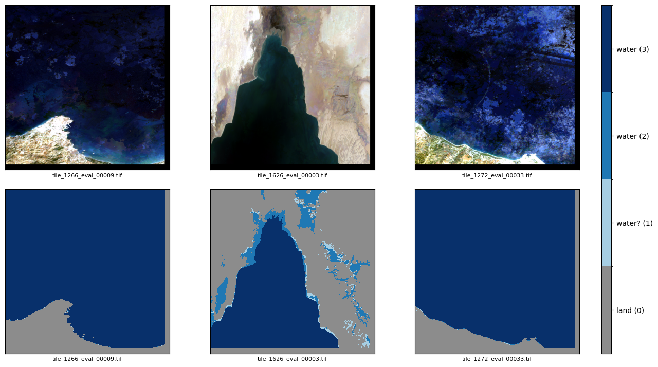
def _read_img_rgb(path):"""Read 4-band image [B2,B3,B4,B5] and return RGB as B4,B3,B2, scaled to [0,1]."""with rio.open(path) as src: arr = src.read() # (C,H,W) = (4,H,W) arr = np.transpose(arr, (1,2,0)) # (H,W,4) rgb = arr[..., [2,1,0]] # B4,B3,B2 (natural color)if rgb.dtype == np.uint8:return rgb.astype(np.float32) /255.0 lo = np.percentile(rgb, 2, axis=(0,1), keepdims=True) hi = np.percentile(rgb, 98, axis=(0,1), keepdims=True)return np.clip((rgb - lo) / (hi - lo +1e-6), 0, 1).astype(np.float32)def _read_mask(path):"""Read a mask and clip values to {0,1,2,3}."""with rio.open(path) as src: m = src.read(1).astype(np.uint8)return np.clip(m, 0, 3)def show_samples(split='train', data_root='dataset_compact', num=3, seed=None, title=False):""" Display random samples (top: RGB, bottom: mask) from a split. Valid splits: 'train' | 'val' | 'eval_tiles' """ split_map = {'train': ('train/images', 'train/masks'),'val': ('val/images', 'val/masks'),'eval_tiles': ('eval_tiles/images', 'eval_tiles/masks'), }if split notin split_map:raiseValueError(f"Unknown split '{split}'. Use one of {list(split_map)}.") img_dir =f"{data_root}/{split_map[split][0]}" msk_dir =f"{data_root}/{split_map[split][1]}" files =sorted(glob.glob(f"{img_dir}/*.tif"))ifnot files:raiseFileNotFoundError(f"No images found in {img_dir}") rng = random.Random(seed if seed isnotNoneelse randbits(64)) sel = rng.sample(files, k=min(num, len(files)))# Discrete colormap for labels: 0=land (gray), 1–3 water confidence (light→dark blue) cmap = ListedColormap(["#8c8c8c", "#a6cee3", "#1f78b4", "#08306b"]) norm = BoundaryNorm([-0.5, 0.5, 1.5, 2.5, 3.5], cmap.N)# Figure with dedicated colorbar column fig = plt.figure(figsize=(4*len(sel)+1, 7), constrained_layout=True) gs = GridSpec(2, len(sel) +1, figure=fig, width_ratios=[1]*len(sel) + [0.05]) axes_img = [fig.add_subplot(gs[0, i]) for i inrange(len(sel))] axes_msk = [fig.add_subplot(gs[1, i]) for i inrange(len(sel))] cax = fig.add_subplot(gs[:, -1]) last_im =Nonefor j, img_path inenumerate(sel): msk_path = img_path.replace("/images/", "/masks/") rgb = _read_img_rgb(img_path) msk = _read_mask(msk_path) ax_img = axes_img[j] ax_img.imshow(rgb) ax_img.set_xticks([]); ax_img.set_yticks([]) ax_img.set_xlabel(img_path.split("/")[-1], fontsize=8, labelpad=4) ax_msk = axes_msk[j] last_im = ax_msk.imshow(msk, cmap=cmap, norm=norm, interpolation="nearest") ax_msk.set_xticks([]); ax_msk.set_yticks([]) ax_msk.set_xlabel(msk_path.split("/")[-1], fontsize=8, labelpad=4)if last_im isnotNone: cbar = fig.colorbar(last_im, cax=cax, ticks=[0,1,2,3]) cbar.ax.set_yticklabels(["land (0)", "water? (1)", "water (2)", "water (3)"]) fig.set_constrained_layout_pads(w_pad=0.02, h_pad=0.03, wspace=0.02, hspace=0.03)if title: fig.suptitle(f"{split} samples (top: RGB B4/B3/B2, bottom: labels 0–3)", y=0.995) plt.show()
Have a look at some of the examples. Note the optional parameter “seed”. If you specify the seed, it will always pick the same random clips. If you don’t (or change the value of the seed), then re-running the same code cell / function call, will select different random clips each time. The RGB data are shown in the top and the masks in the bottom row. You’ll see that the labels are still 0 for land, and 1 for “maybe” water, 2 for “probably” water, and 3 for “definitely” water, with a colorbar legend on the right.
Code
# Just running the function will tell you wat inputs it expects / allows for.show_samples
/tmp/ipython-input-2193594441.pyDisplay random samples (top: RGB, bottom: mask) from a split.
Valid splits: 'train' | 'val' | 'eval_tiles'
👉 Try it yourself: play with some of the options to get a sense of what our training data looks like.
❓ Question: Do you notice any differences when looking at the train/val data as compared to the eval_tiles data?
Code
# show_samples('val', num=4, seed=123) # reproducible selection# show_samples('train', num=3) # new random each run# show_samples('eval_tiles', num=3, seed=123) # from eval_tiles
Answer to the previous question: You may have noticed/remembered that the evaluation clips are about $3$ larger than the training/validation clips, so they may show a bit more complexity in the water morphologies than the more “zoomed in” smaller clips. Also, the larger clips have some padding on the right and bottom. This is because the source I used ( https://github.com/giswqs/deep-water-map ) has clips of 743 \(\times\) 744 but it is more convenient, or necessary depending on the ML algorithm, if the output is a multiple of our training clips 256 \(\times\) 256 (specifically, 3\(\times\) in each direction).
Code
show_samples('eval_tiles', num=3, seed=123) # from eval_tiles
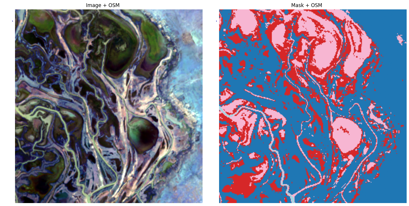
Here’s another function that was intended to also add an Open Street Map (OSM) layer to show where the images are located in the Arctic, but it doesn’t quite work as intended yet (the image is on top of the OSM, so you can’t see it; the idea was for the OSM map to be larger than the satellite image clip). You can skip this (or try to fix it ;) ).
Code
def plot_clip_with_vector_osm(base_dir, feature_types=("water", "roads")):""" Pick a random clip from train/val/eval folders and plot image+mask with OSM overlays. """# --- pick random clip img_dir = os.path.join(base_dir, "images") mask_dir = os.path.join(base_dir, "masks") img_file = random.choice(sorted(os.listdir(img_dir))) img_path = os.path.join(img_dir, img_file) mask_path = os.path.join(mask_dir, img_file)# --- read datawith rasterio.open(img_path) as src: img = src.read([1, 2, 3]) # RGB bands img = img.transpose(1, 2, 0) img_bounds = src.bounds img_crs = src.crswith rasterio.open(mask_path) as src: mask = src.read(1)# --- reproject bounds to WGS84 for OSM transformer = Transformer.from_crs(img_crs, "EPSG:4326", always_xy=True) minx, miny = transformer.transform(img_bounds.left, img_bounds.bottom) maxx, maxy = transformer.transform(img_bounds.right, img_bounds.top)# pad the bbox to improve OSM queries pad_x = (maxx - minx) *0.5 pad_y = (maxy - miny) *0.5 poly_wgs = box(minx - pad_x, miny - pad_y, maxx + pad_x, maxy + pad_y)# --- get correct API function depending on osmnx versionif version.parse(ox.__version__) >= version.parse("2.0"): get_geoms = ox.features_from_polygonelse: get_geoms = ox.geometries.geometries_from_polygondef safe_get_geoms(tags):try:return get_geoms(poly_wgs, tags=tags)except InsufficientResponseError:returnNone# --- download features gdfs = {}if"water"in feature_types: gdfs["water"] = safe_get_geoms({"natural": "water"})if"roads"in feature_types: gdfs["roads"] = safe_get_geoms({"highway": True})# --- plot fig, axes = plt.subplots(1, 2, figsize=(14, 7)) ax_img, ax_mask = axes ax_img.imshow(img / img.max()) # normalize for plotting ax_img.set_title("Image + OSM") ax_img.axis("off") ax_mask.imshow(mask, cmap="tab20") ax_mask.set_title("Mask + OSM") ax_mask.axis("off")# overlay OSM layersfor name, gdf in gdfs.items():if gdf isnotNoneandnot gdf.empty:if name =="water": gdf.plot(ax=ax_img, facecolor="none", edgecolor="blue", linewidth=1, alpha=0.5) gdf.plot(ax=ax_mask, facecolor="none", edgecolor="blue", linewidth=1, alpha=0.5)if name =="roads": gdf.plot(ax=ax_img, color="black", linewidth=0.8, alpha=0.7) gdf.plot(ax=ax_mask, color="black", linewidth=0.8, alpha=0.7) plt.tight_layout() plt.show()plot_clip_with_vector_osm("dataset_compact/train", feature_types=("water","roads"))
Code
Data pre-processing
Recap question: What is the difference between 8-bit and 16-bit imagery?
Click here for the answer
An 8-bit image can represent \[2^8 = 256\]
discrete intensity levels (values 0–255).
A 16-bit image can represent \[2^{16} = 65,536\]
discrete intensity levels (values 0–65,535).
If we assume reflectance values are scaled into the range \([0,1]\):
So 16-bit data has ~256× finer precision than 8-bit.
This matters in scientific imagery (e.g. remote sensing), where subtle reflectance differences can be lost if the data are quantized to only 256 levels.
In short:
- 8-bit: good for display and simple tasks.
- 16-bit: essential for preserving detail, avoiding banding, and keeping dynamic range for analysis.
Let’s explicitly check again what the properties of our dataset are.
❓ Question: Do you know enough linux/bash or can you find out with google/chatgpt how to get the full path of the first (or, really, any) image in the folder of training image clips?
Hint/answer
!ls dataset_compact/train/images/ file is: tile_1204_train_i000161.tif
Here I provide an example of how one way to use the python libraries rioxarray or rasterio to read the geotiff file into an xarray, which is given the variable name arr below. xarray allows many of the same operations as on standard numpy arrays, but it also preserves the geospatial information. Specifically, each pixel doesn’t just have a value of RGB-NIR reflectances, but it also has associated lat/lon coordiate information and the xarray has metadata for coordinate reference information etc.
Code
# I find rioxarray the most straightforward approach:first_file =""# you need to find and plug in the full path to any of the train/eval image clipsxarr = rioxarray.open_rasterio(first_file)
---------------------------------------------------------------------------KeyError Traceback (most recent call last)
/usr/local/lib/python3.12/dist-packages/xarray/backends/file_manager.py in _acquire_with_cache_info(self, needs_lock) 218try:--> 219file = self._cache[self._key] 220except KeyError:/usr/local/lib/python3.12/dist-packages/xarray/backends/lru_cache.py in __getitem__(self, key) 55with self._lock:---> 56value = self._cache[key] 57 self._cache.move_to_end(key)KeyError: [<function open at 0x7de4732c36a0>, ('',), 'r', (('sharing', False),), 'c8e6b598-cb42-4ddb-b71b-9d01fa37a19e']
During handling of the above exception, another exception occurred:
CPLE_OpenFailedError Traceback (most recent call last)
rasterio/_base.pyx in rasterio._base.DatasetBase.__init__()rasterio/_base.pyx in rasterio._base.open_dataset()rasterio/_err.pyx in rasterio._err.exc_wrap_pointer()CPLE_OpenFailedError: : No such file or directory
During handling of the above exception, another exception occurred:
RasterioIOError Traceback (most recent call last)
/tmp/ipython-input-4067998613.py in <cell line: 0>() 3 first_file =""# you need to find and plug in the full path to any of the train/eval image clips 4----> 5xarr = rioxarray.open_rasterio(first_file)/usr/local/lib/python3.12/dist-packages/rioxarray/_io.py in open_rasterio(filename, parse_coordinates, chunks, cache, lock, masked, mask_and_scale, variable, group, default_name, decode_times, decode_timedelta, band_as_variable, **open_kwargs) 1133else: 1134 manager = URIManager(file_opener, filename, mode="r", kwargs=open_kwargs)-> 1135riods = manager.acquire() 1136 captured_warnings = rio_warnings.copy() 1137/usr/local/lib/python3.12/dist-packages/xarray/backends/file_manager.py in acquire(self, needs_lock) 199 An open file object,as returned by``opener(*args,**kwargs)``. 200 """
--> 201file, _ = self._acquire_with_cache_info(needs_lock) 202return file
203/usr/local/lib/python3.12/dist-packages/xarray/backends/file_manager.py in _acquire_with_cache_info(self, needs_lock) 223 kwargs = kwargs.copy() 224 kwargs["mode"]= self._mode
--> 225file = self._opener(*self._args,**kwargs) 226if self._mode =="w": 227# ensure file doesn't get overridden when opened again/usr/local/lib/python3.12/dist-packages/rasterio/env.py in wrapper(*args, **kwds) 461 462with env_ctor(session=session):--> 463return f(*args,**kwds) 464 465return wrapper
/usr/local/lib/python3.12/dist-packages/rasterio/__init__.py in open(fp, mode, driver, width, height, count, crs, transform, dtype, nodata, sharing, opener, **kwargs) 354 355if mode =="r":--> 356dataset = DatasetReader(path, driver=driver, sharing=sharing,**kwargs) 357elif mode =="r+": 358 dataset = get_writer_for_path(path, driver=driver)(
rasterio/_base.pyx in rasterio._base.DatasetBase.__init__()RasterioIOError: : No such file or directory
Check all the information contained in such an xarray:
Code
print("Xarray object with metadata:")print(xarr)print("\nAttributes (metadata):")print(xarr.attrs)print("\n\n\nCoordinates (note: these include spatial info):")print(xarr.coords)# To get min/max per bandfor i inrange(xarr.sizes["band"]): band_data = xarr.isel(band=i)print(f"Band {i+1}: min={band_data.min().item()}, max={band_data.max().item()}")
Below is a different library but almost the same approach to achieve the same thing using rasterio rather than rioxarray (similar packages):
Code
first_file =""# fill in; this can be any image clip in the train or eval foldersprint("Opening:", first_file)with rio.open(first_file) as src: arr = src.read() # shape = (bands, height, width)print("Shape (bands, height, width):", arr.shape)# Loop through bandsfor i inrange(arr.shape[0]): band = arr[i]print(f"Band {i+1}: min={band.min()}, max={band.max()}")
Feature engineering
Once again, the reflectances of the Landsat (or Sentinel) images for each pixel are the features for this ML/DL task.
❓ Question: Are these features suitable for a ML/DL algorithm for logistic classification as-is?
If not, why not, and how should we change those?
Hint
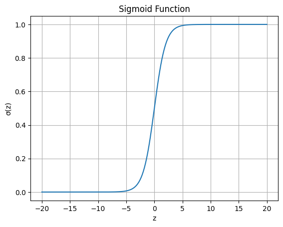
Think about the sigmoid activation function in logistic regression:
\[
\sigma(z) = \frac{1}{1 + e^{-z}}, \quad z = \mathbf{w}^\top \mathbf{x} + b
\]
What happens if \(x\) is very large (like reflectance 199)?
Hint/answer
Large reflectance values make (z) very large, so ((z)) saturates to 1 (or 0).
This kills the gradient updates and breaks learning.
👉 We should scale reflectances before feeding them into logistic regression or other ML/DL models.
Common approaches:
- Min–max scaling to [0–1]
- Percentile stretch (2–98%) followed by [0–1] normalization
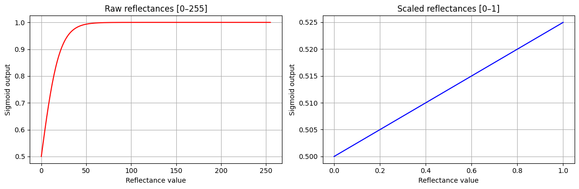
Here’s a basic demo of how the sigmoid function quickly saturates when using raw 8-bit reflectances (this would be even way worse for the original 16-bit reflectance values), while it behaves much better for normalized reflectance inputs.
Code
reflectance_raw =int(input("Enter a reflectance value between 0 and 255: "))weight =0.1bias =0.0z_raw = weight * reflectance_raw + biassig_raw = sigmoid(z_raw)reflectance_scaled = reflectance_raw /255.0z_scaled = weight * reflectance_scaled + biassig_scaled = sigmoid(z_scaled)print(f"\nRaw reflectance = {reflectance_raw}")print(f" z = {z_raw:.2f}, sigmoid(z) = {sig_raw:.6f}")print(f"\nScaled reflectance = {reflectance_scaled:.3f}")print(f" z = {z_scaled:.6f}, sigmoid(z) = {sig_scaled:.6f}")
Enter a reflectance value between 0 and 255: 89

Raw reflectance = 89
  z = 8.90, sigmoid(z) = 0.999864

Scaled reflectance = 0.349
  z = 0.034902, sigmoid(z) = 0.508725
Here’s a more visual illustration for just the positive range of the sigmoid function and some initial guess of fitted weight and bias:
Code
w =0.1bias =0.0# Case 1: raw reflectances [0,255]x_raw = np.linspace(0, 255, 256)z_raw = w * x_raw + biassig_raw = sigmoid(z_raw)# Case 2: scaled reflectances [0,1]x_scaled = np.linspace(0, 1, 256)z_scaled = w * x_scaled + biassig_scaled = sigmoid(z_scaled)fig, axes = plt.subplots(1, 2, figsize=(12, 4))axes[0].plot(x_raw, sig_raw, color="red")axes[0].set_title("Raw reflectances [0–255]")axes[0].set_xlabel("Reflectance value")axes[0].set_ylabel("Sigmoid output")axes[0].grid(True)axes[1].plot(x_scaled, sig_scaled, color="blue")axes[1].set_title("Scaled reflectances [0–1]")axes[1].set_xlabel("Reflectance value")axes[1].set_ylabel("Sigmoid output")axes[1].grid(True)plt.tight_layout()plt.show()
Play around with the cell below to practice these different feature re-scaling ideas.
Code
# 👉 Step 1. Pick any image clip from your dataset (train/val/eval)# first_file = "" # <-- fill in with full path to an image, e.g. "dataset_compact/train/images/<>.tif"# Open with rioxarray (bands, height, width)xarr = rioxarray.open_rasterio(first_file)print("Raw shape (bands, H, W):", xarr.shape)print("Data type:", xarr.dtype)print("Raw min/max reflectance values:", float(xarr.min()), float(xarr.max()))# --------------------------------------# Once again, remember: each pixel’s reflectances in the 4 bands are the *features*.## ❓ Question:# Are the raw integer reflectances in the 0–255 range directly suitable# for logistic regression or deep learning?## Hint: Think about how the sigmoid behaves for very large vs. small inputs.# --------------------------------------# Step 2. Flatten the array into (H, W, C) form for easier handlingimg = xarr.transpose("y", "x", "band").valuesprint("Reordered shape (H, W, C):", img.shape)# Step 3. Explore percentile-based reflectance scaling# 👉 Compute the 2% and 98% percentiles across all pixels:lo = np.percentile(img, 2, axis=(0,1))hi = np.percentile(img, 98, axis=(0,1))print("Per-band 2% percentiles:", lo)print("Per-band 98% percentiles:", hi)# ❓ Question:# For 8-bit reflectances (0–255), what do you expect these values to be close to?# (Think: about 5 for low, 250 for high).# This is why in our universal scaling we just fix low=5, high=250.# Step 4. Apply clippingimg_clipped = np.clip(img, 5, 250)print("After clipping → min:", img_clipped.min(), "max:", img_clipped.max())# Step 5. Normalize to [0,1]img_norm = (img_clipped -5) / (250-5)print("After normalization → min:", img_norm.min(), "max:", img_norm.max())# --------------------------------------# 👉 Suggestion:# Print out min/max again after each step.# Try plotting histograms of reflectance values to *see* the effect# of clipping and scaling.# --------------------------------------# Step 6. Process the mask file in a similar waymask_file = first_file.replace("/images/", "/masks/")mask = rioxarray.open_rasterio(mask_file).values.squeeze()print("Mask shape:", mask.shape, "unique labels:", np.unique(mask))# ❓ Question:# How can we collapse the 4 classes {0,1,2,3} into just land vs. water?# Hint: np.where( np.isin(mask, [2,3]), 1, 0 )
---------------------------------------------------------------------------KeyError Traceback (most recent call last)
/usr/local/lib/python3.12/dist-packages/xarray/backends/file_manager.py in _acquire_with_cache_info(self, needs_lock) 218try:--> 219file = self._cache[self._key] 220except KeyError:/usr/local/lib/python3.12/dist-packages/xarray/backends/lru_cache.py in __getitem__(self, key) 55with self._lock:---> 56value = self._cache[key] 57 self._cache.move_to_end(key)KeyError: [<function open at 0x7de4732c36a0>, ('',), 'r', (('sharing', False),), '57f65f9f-fbbd-4e8e-819e-6b305c1e14e6']
During handling of the above exception, another exception occurred:
CPLE_OpenFailedError Traceback (most recent call last)
rasterio/_base.pyx in rasterio._base.DatasetBase.__init__()rasterio/_base.pyx in rasterio._base.open_dataset()rasterio/_err.pyx in rasterio._err.exc_wrap_pointer()CPLE_OpenFailedError: : No such file or directory
During handling of the above exception, another exception occurred:
RasterioIOError Traceback (most recent call last)
/tmp/ipython-input-2545844640.py in <cell line: 0>() 3 4# Open with rioxarray (bands, height, width)----> 5xarr = rioxarray.open_rasterio(first_file) 6 print("Raw shape (bands, H, W):", xarr.shape) 7 print("Data type:", xarr.dtype)/usr/local/lib/python3.12/dist-packages/rioxarray/_io.py in open_rasterio(filename, parse_coordinates, chunks, cache, lock, masked, mask_and_scale, variable, group, default_name, decode_times, decode_timedelta, band_as_variable, **open_kwargs) 1133else: 1134 manager = URIManager(file_opener, filename, mode="r", kwargs=open_kwargs)-> 1135riods = manager.acquire() 1136 captured_warnings = rio_warnings.copy() 1137/usr/local/lib/python3.12/dist-packages/xarray/backends/file_manager.py in acquire(self, needs_lock) 199 An open file object,as returned by``opener(*args,**kwargs)``. 200 """
--> 201file, _ = self._acquire_with_cache_info(needs_lock) 202return file
203/usr/local/lib/python3.12/dist-packages/xarray/backends/file_manager.py in _acquire_with_cache_info(self, needs_lock) 223 kwargs = kwargs.copy() 224 kwargs["mode"]= self._mode
--> 225file = self._opener(*self._args,**kwargs) 226if self._mode =="w": 227# ensure file doesn't get overridden when opened again/usr/local/lib/python3.12/dist-packages/rasterio/env.py in wrapper(*args, **kwds) 461 462with env_ctor(session=session):--> 463return f(*args,**kwds) 464 465return wrapper
/usr/local/lib/python3.12/dist-packages/rasterio/__init__.py in open(fp, mode, driver, width, height, count, crs, transform, dtype, nodata, sharing, opener, **kwargs) 354 355if mode =="r":--> 356dataset = DatasetReader(path, driver=driver, sharing=sharing,**kwargs) 357elif mode =="r+": 358 dataset = get_writer_for_path(path, driver=driver)(
rasterio/_base.pyx in rasterio._base.DatasetBase.__init__()RasterioIOError: : No such file or directory
✅ Takeaways:
- Raw 8-bit reflectances (0–255) → saturate sigmoid, bad for learning.
- Simple min–max scaling (0–1) → much better, keeps values in a useful range.
- Best practice:
Apply a 2–98% percentile stretch to remove outliers, then normalize to [0–1].
This makes features more robust and keeps ML/DL models stable.
To get everyone on the same page moving forward, below is a clean function that does all the required pre-processing on all of the training and validation data in terms of min-max scaling and percentile stretching. It also converts the land-water labels 0, 1, 2, 3 into just binary labels 0 (land) and 1 (water). Finally, I added an option frac_data, which is simply the fraction of our total amount of available training and validation data to use. The default is frac_data=1.0, using all data. For frac_data=0.1, we’d use 100 training images and 20 validation images. This is useful for faster results and in cases where Colab might run out of memory otherwise.
Code
def load_data_and_collapse(base_dir, low=5, high=250, frac_data=1.0, seed=0):""" Load image+mask pairs from a folder, preprocess, flatten into feature vectors, and return X (features) and y (binary labels). Parameters ---------- base_dir : str Path to folder with 'images/' and 'masks/' subfolders low, high : int Fixed scaling range for reflectances (default [5, 250]) frac_data : float, optional Fraction of image/mask pairs to use (default 1.0 = all). E.g., 0.1 uses only 10% of available pairs. seed : int, optional Random seed for reproducibility when selecting a subset. Returns ------- X : np.ndarray, shape (N_pixels, N_bands) Flattened features across all selected images y : np.ndarray, shape (N_pixels,) Flattened binary labels across all selected images """ img_files =sorted(glob.glob(f"{base_dir}/images/*.tif")) mask_files =sorted(glob.glob(f"{base_dir}/masks/*.tif"))# --- Optionally subsample the dataset --- n_files =len(img_files) n_select =max(1, int(frac_data * n_files)) rng = random.Random(seed) idx_select =sorted(rng.sample(range(n_files), n_select)) img_files = [img_files[i] for i in idx_select] mask_files = [mask_files[i] for i in idx_select] X_list, y_list = [], []for img_path, mask_path inzip(img_files, mask_files):# --- Load image --- img = rioxarray.open_rasterio(img_path) # (bands, H, W) img = img.transpose("y", "x", "band").values # (H, W, C)# Scale reflectances: 5 → 0, 250 → 1 img = np.clip((img - low) / (high - low), 0, 1)# --- Load mask --- mask = rioxarray.open_rasterio(mask_path).values.squeeze() # (H, W)# Collapse labels: (0+1 → 0 land), (2+3 → 1 water) mask_bin = np.where(np.isin(mask, [2, 3]), 1, 0)# --- Flatten --- X_list.append(img.reshape(-1, img.shape[-1])) y_list.append(mask_bin.ravel())# --- Concatenate across all images --- X = np.vstack(X_list) y = np.hstack(y_list)return X, y
Linear logistic regression
Using the function that we create at the end of the Feature Engineering section, let’s load our training and validation data and pre-process them with min-max scaling and percentile stretching:
Code
# Example: load training and validation datat0 = time.time()X_train, y_train = load_data_and_collapse("dataset_compact/train",frac_data=0.1)X_val, y_val = load_data_and_collapse("dataset_compact/val",frac_data=0.1)print(f"Data loaded in {time.time()-t0:.2f} seconds")# Shapesprint("Train features:", X_train.shape) # (N_pixels_total, N_bands)print("Train labels: ", y_train.shape) # (N_pixels_total,)print("Val features: ", X_val.shape)print("Val labels: ", y_val.shape)# Peek at rangesprint("Feature range (train): min =", X_train.min(), ", max =", X_train.max())print("Unique labels in train:", np.unique(y_train))
Data loaded in 3.15 seconds
Train features: (6553600, 4)
Train labels:   (6553600,)
Val features:   (1310720, 4)
Val labels:     (1310720,)
Feature range (train): min = 0.0 , max = 1.0
Unique labels in train: [0 1]
Training a linear logistic regression model is again deceptively simple if we use the off-the-shelf black box functions from scikit-learn. Specifically, we’ll use LogisticRegression. As explained in earlier labs, these function actually do various optimization internally that you may not always be aware of. In this case, LogisticRegression actually already does some sorts of feature scaling internally to perform better, i.e. it does not only just do a basic regression. It also already uses regularization by default to avoid overfitting. You can learn about some of this by simply typing
? LogisticRegression
in a code cell.
In a later step, I’ll show you again how to achieve the same ‘from scratch’ with just plain algebra and no black box libraries.
Code
# Fit logistic regressiont1 = time.time()clf = LogisticRegression(max_iter=200, n_jobs=-1)clf.fit(X_train, y_train)print(f"Training done in {time.time()-t1:.2f} s")
Training done in 11.44 s
Acknowledge how insane it is that we can train this model in just seconds! Remember from the earlier prompts/questions how many input variables/features we are processing, and we’re not even using a GPU yet.
At this point, our model which we named clf for classification only contains the “fitting parameters” of our best logistic regression fit to our labeled images. All the way in the top, we also loaded another very convenient scikit-learn function: from sklearn.metrics import classification_report. Let’s first see how this works to see how well our trained model fits the training data itself:
Remember that the f1-score is the (harmonic) average of precision and recall. The harmonic average is close to the lower value of whatever is averaged, so it is a single conservative metric of performance. What do you see for the overall accuracy in classifying water pixels from RGB-NIR Landsat satellite imagery using our linear logistic regression model?
Pretty great for such a simple model, right?
To my surprise, I accidentally discovered in putting this lab together that the LogisticRegression function actually performs significantly better when we don't do the usual best-practice feature scaling. The reasons are a bit complicated but have to do, again, with various other steps that are hidden inside this function. For example, it uses a “L2 regularized solver” by default rather than the typical gradient-based method, and by scaling from 0-255 to 5-250 and then normalizing, we lost some of the range in the raw data.
Below, we train LogisticRegression again but just on the raw image data.
First, a near identical function to just load the image + mask data without feature scaling:
Code
def load_raw_reflectances(base_folder, frac_data=1.0, seed=0):""" Load image/mask pairs and collapse labels into binary (land=0, water=1). Returns raw reflectance values (0–255), no scaling. Parameters ---------- base_folder : str Path to folder with 'images/' and 'masks/' subfolders frac_data : float, optional Fraction of image/mask pairs to use (default 1.0 = all). E.g., 0.1 uses only 10% of available pairs. seed : int, optional Random seed for reproducibility when selecting a subset. Returns ------- X_out : np.ndarray, shape (N_pixels, N_bands) Flattened features across selected images y_out : np.ndarray, shape (N_pixels,) Flattened binary labels across selected images """ image_files =sorted(glob.glob(f"{base_folder}/images/*.tif")) mask_files =sorted(glob.glob(f"{base_folder}/masks/*.tif"))# --- Optionally subsample dataset --- n_files =len(image_files) n_select =max(1, int(frac_data * n_files)) rng = random.Random(seed) idx_select =sorted(rng.sample(range(n_files), n_select)) image_files = [image_files[i] for i in idx_select] mask_files = [mask_files[i] for i in idx_select] features_all, labels_all = [], []for img_file, mask_file inzip(image_files, mask_files):# --- Load image --- img = rioxarray.open_rasterio(img_file).values.transpose(1, 2, 0) # (H, W, C)# --- Load mask --- mask = rioxarray.open_rasterio(mask_file).values[0] # single band# Collapse labels: (0,1) → 0 (land), (2,3) → 1 (water) mask_binary = np.where(np.isin(mask, [2, 3]), 1, 0)# Flatten features_all.append(img.reshape(-1, img.shape[-1])) labels_all.append(mask_binary.ravel()) X_out = np.vstack(features_all) y_out = np.hstack(labels_all)return X_out, y_out
Code
# --- Load training and validation sets (raw reflectances) ---t0 = time.time()X_train_raw, y_train_raw = load_raw_reflectances("dataset_compact/train", frac_data=0.1)X_val_raw, y_val_raw = load_raw_reflectances("dataset_compact/val", frac_data=0.1)print(f"Raw data loaded in {time.time()-t0:.2f} s")# --- Fit logistic regression (on raw reflectances) ---t1 = time.time()clf_raw = LogisticRegression(max_iter=200, n_jobs=-1)clf_raw.fit(X_train_raw, y_train_raw)print(f"Training done in {time.time()-t1:.2f} s")# --- Evaluate on validation set ---t2 = time.time()y_val_pred_raw = clf_raw.predict(X_val_raw)print(f"Prediction done in {time.time()-t2:.2f} s")print("\nClassification report (binary land=0, water=1):")print(classification_report(y_val_raw, y_val_pred_raw))
Raw data loaded in 2.11 s
Training done in 15.15 s
Prediction done in 0.04 s

Classification report (binary land=0, water=1):
              precision    recall  f1-score   support

           0       0.96      0.96      0.96    844951
           1       0.93      0.92      0.92    465769

    accuracy                           0.95   1310720
   macro avg       0.94      0.94      0.94   1310720
weighted avg       0.95      0.95      0.95   1310720
These results are quite amazing!
👉 Assignment: Load a single image and mask from the eval_tiles folder, perform inference/prediction on that image, and compute the error/accuracy metrics versus the corresponding mask of ground-truth labels.
👉 Assignment: Generalize the previous code to loop through each image/mask pair in the eval_tiles folder and print out the accuracy metrics.
Code
# Write your own code here to make a prediction for the larger 768x768 tiles in eval_tiles# first for just one clip and then for multiple/all# Analyze how well our model performs on those larger images.
💡 Hint 1: Single eval tile
# pick a single eval image + maskimg_path ="dataset_compact/eval_tiles/images/<filename>.tif"mask_path ="dataset_compact/eval_tiles/masks/<filename>.tif"# load image and maskimg = rioxarray.open_rasterio(img_path).values.transpose(1,2,0)mask = rioxarray.open_rasterio(mask_path).values[0]# collapse labels to binarymask_bin = np.where(np.isin(mask, [2,3]), 1, 0)# flattenX_eval = img.reshape(-1, img.shape[-1])y_eval = mask_bin.ravel()# predict with trained classifiery_pred_eval = clf_raw.predict(X_eval) # or clf if using scaled version# metricsprint(classification_report(y_eval, y_pred_eval))
💡 Hint 2: Loop through all eval tiles
image_files =sorted(glob.glob("dataset_compact/eval_tiles/images/*.tif"))mask_files =sorted(glob.glob("dataset_compact/eval_tiles/masks/*.tif"))for img_path, mask_path inzip(image_files, mask_files):# load img = rioxarray.open_rasterio(img_path).values.transpose(1,2,0) mask = rioxarray.open_rasterio(mask_path).values[0] mask_bin = np.where(np.isin(mask, [2,3]), 1, 0)# flatten X_eval = img.reshape(-1, img.shape[-1]) y_eval = mask_bin.ravel()# predict y_pred_eval = clf_raw.predict(X_eval) # or clf if using scaled version# print metrics per tileprint(f"\nResults for {img_path.split('/')[-1]}:")print(classification_report(y_eval, y_pred_eval, digits=3))
Helpful functions
The below actually implements what the previous lab exercise/question was. It adds one more option.
As outlined in the very beginning, the training images for DeepWaterLab had somewhat inconvenient and non-consistent pixel dimension of \(743 \times 744\), \(744\times 743\), \(744\times 744\). Especially for convolutional neural networks, CNN, it is useful/necessary to have standard dimenions as powers of 2 or in our case also multiples or our training tiles. For these reasons, I “padded” these images to \(3\times 256 = 768\) pixels in each dimension. However, those padded pixels have no meaning. So in the functions below, I strip those back out and only make predictions and associated error metrics on the pixels that we actually part of the Landsat images. Actually, we can crop to anything \(<743\) pixels in each dimension. In the examples I pick \(740 \times 740\) pixels.
Code
CROP =740# crop size on larger evaluation images
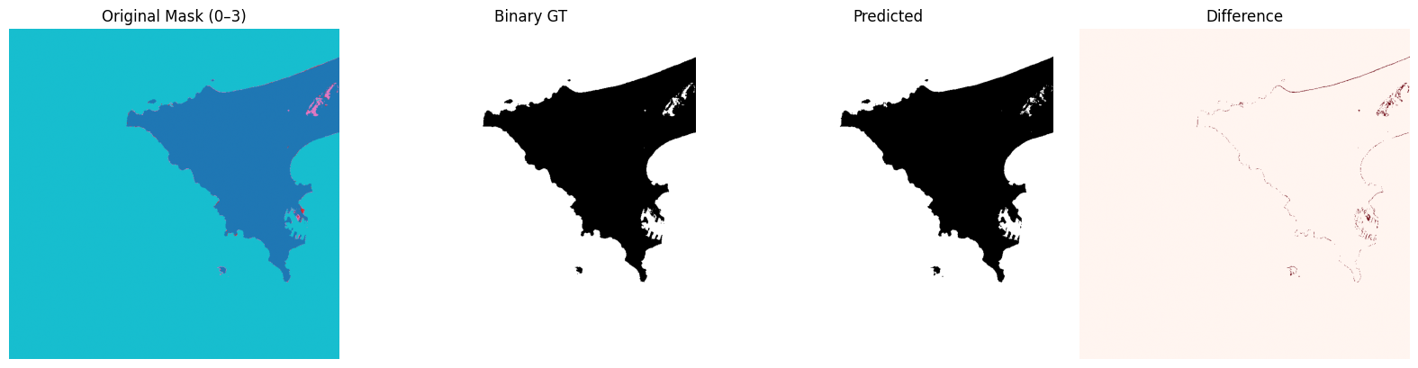
The next function randomy selects one of the larger evaluation images, shows the mask with soft-labels, the mask with binary labels, our model prediction, and a difference map. Then it also prints out the precision/recall/f1-score for just that one selected test image.
Alright, let’s run this over all 50 larger images in the evaluation folder and print a detailed report on precision, recall, and f1 scores. We can do this for either the model that was trained on the pre-processed training data (cfl) or the model trained on the raw data (clf_raw).
Next, let’s see what we can do with logistic regression implemented from scratch using only linear algebra and basic python, just like you learned in earlier weeks.
Logistic regression from-scratch, without skikit-learn / black box
Below I repeat a version of our earlier code for linear logistic regression. I’ll keep the code extremely simple and explicit with minimal use of functions and not even bothering with vectorizing the weights/slopes + bias terms together (which is more efficient).
I did add automatic stopping: after each iteration we check how much the error/loss function has decreased. If it doesn’t decrease anymore within a user defined tolerance (the input tol=1e-4 by default), then we exit the gradient descent loop.
Code
# def compute_loss(y, y_pred):# """Binary cross-entropy loss."""# m = len(y)# return -(1/m) * np.sum(# y * np.log(y_pred + 1e-9) + (1 - y) * np.log(1 - y_pred + 1e-9)# )# ------------------------# Logistic Regression Training (SGD / Mini-batch + Early Stopping)# ------------------------def train_logistic_regression(X, y, learning_rate=0.01, num_iterations=10, batch_size=32, tol=1e-4, patience=3):""" Train logistic regression using mini-batch gradient descent. Includes early stopping and timing info. """ m, n = X.shape weights = np.random.randn(n) *0.01 bias =0.0 best_loss =float('inf') no_improve =0 start_time_total = time.time()for epoch inrange(num_iterations): epoch_start = time.time()# Shuffle the data each epoch indices = np.arange(m) np.random.shuffle(indices) X_shuffled, y_shuffled = X[indices], y[indices]# Mini-batch loopfor i inrange(0, m, batch_size): X_batch = X_shuffled[i:i+batch_size] y_batch = y_shuffled[i:i+batch_size]# Forward pass linear = np.dot(X_batch, weights) + bias y_pred =1/ (1+ np.exp(-linear)) # sigmoid# Gradients error = y_pred - y_batch grad_w = (1/len(y_batch)) * np.dot(X_batch.T, error) grad_b = (1/len(y_batch)) * np.sum(error)# Update weights -= learning_rate * grad_w bias -= learning_rate * grad_b# Evaluate full loss at end of epoch y_pred_full =1/ (1+ np.exp(-(np.dot(X, weights) + bias))) loss =-(1/m) * np.sum( y * np.log(y_pred_full +1e-9) + (1- y) * np.log(1- y_pred_full +1e-9) ) epoch_end = time.time()print(f"Epoch {epoch+1}/{num_iterations}, "f"Loss: {loss:.4f}, "f"Time: {epoch_end - epoch_start:.2f} sec")# Early stopping checkif loss + tol < best_loss: best_loss = loss no_improve =0else: no_improve +=1if no_improve >= patience:print(f"Stopping early at epoch {epoch+1} "f"(no improvement for {patience} epochs).")break total_end = time.time()print(f"\nTraining completed in {total_end - start_time_total:.2f} seconds.\n")return weights, bias# ------------------------# Prediction# ------------------------def predict_labels(X, weights, bias, threshold=0.5):"""Predict binary labels (0 or 1) given learned weights and bias.""" linear = np.dot(X, weights) + bias probs = sigmoid(linear)return (probs >= threshold).astype(int)
Define a fancy “class” for this model. In a nutshell, a class lets us group various variable definitions and functions together into one object. A practical implication is that this allows us to swap out our own logistic regression exactly like how scikit-learn’s logisticregression function was used.
Code
# ------------------------# Training wrapper# This defines a python "class". Don't worry too much about how that works# (or ask chatgpt for some explanation!)# ------------------------class SimpleLogisticRegressionScratch:"""Wrapper to look like sklearn's LogisticRegression"""def__init__(self, learning_rate=0.1, num_iterations=1000):self.learning_rate = learning_rateself.num_iterations = num_iterationsself.feature_weights =Noneself.bias_term =Nonedef fit(self, X, y):self.feature_weights, self.bias_term = train_logistic_regression( X, y, learning_rate=self.learning_rate, num_iterations=self.num_iterations )def predict(self, X):return predict_labels(X, self.feature_weights, self.bias_term)
Code
# -------------------------# Load a subset of training and validation data (scaled reflectances)# -------------------------X_train_small, y_train_small = load_data_and_collapse("dataset_compact/train", low=5, high=250, frac_data=0.1# take only 10% of training clips)X_val_scaled, y_val = load_data_and_collapse("dataset_compact/val", low=5, high=250, frac_data=0.1# take only 10% of validation clips)# -------------------------# Train logistic regression from scratch# -------------------------scratch_model = SimpleLogisticRegressionScratch( learning_rate=0.1, num_iterations=50)scratch_model.fit(X_train_small, y_train_small)# Predict on validation sety_val_pred = scratch_model.predict(X_val_scaled)# Report metrics on validation setprint("Classification report on validation set (from scratch):")print(classification_report(y_val, y_val_pred))
Epoch 1/50, Loss: 0.5259, Time: 7.32 sec
Epoch 2/50, Loss: 0.5247, Time: 5.73 sec
Epoch 3/50, Loss: 0.5253, Time: 7.39 sec
Epoch 4/50, Loss: 0.5247, Time: 5.69 sec
Epoch 5/50, Loss: 0.5246, Time: 7.46 sec
Stopping early at epoch 5 (no improvement for 3 epochs).

Training completed in 33.60 seconds.

Classification report on validation set (from scratch):
              precision    recall  f1-score   support

           0       0.87      0.96      0.91    844951
           1       0.90      0.74      0.81    465769

    accuracy                           0.88   1310720
   macro avg       0.89      0.85      0.86   1310720
weighted avg       0.88      0.88      0.88   1310720
👉 Quiz: What are the hyperparameters a user can play with in this setup?
💡 Show Answer
Learning rate (how big each step is during gradient descent).
Fraction of training data used (frac_data parameter when loading).
Lower and upper percentiles for feature scaling (e.g. 2% → value ≈ 5, 98% → value ≈ 250).
👉 Assignment: Adjust each hyperparameter and observe how it changes the results in both computational cost and final performance/accuracy.
💡 Hints
Try different learning rates (e.g. 0.01, 0.1, 1.0) and see how quickly or poorly the model converges.
Change the fraction of training data (frac_data=0.05, 0.1, 0.5, 1.0) to balance speed vs accuracy.
Modify the feature scaling bounds (e.g. low=1, high=254 vs low=5, high=250) and see how this affects stability and performance.
👉 Question: What did you find when testing different scaling bounds?
💡 Show Answer
You should have found that in this case the stretching of the spectral bands between some lower and upper percentile actually results in poorer results.
The best performance may occur when using the full raw range (low=0, high=255).
Why does this happen?
- For models like logistic regression with built-in regularization, rescaling the data can shrink feature values.
- Smaller features → smaller weights → regularization penalty dominates → the model underfits.
- In other words: while percentile-based scaling is often a “best practice” for noisy, heterogeneous datasets, here the raw reflectance values (0–255) already provide a meaningful spread.
- Neural networks might still benefit from percentile scaling, but this simple linear model actually performed better with the unscaled reflectances.
Convolutional Neural Network
🧠 U-Net: Convolutional Neural Network for Image Segmentation
U-Net is a type of Convolutional Neural Network (CNN) designed for semantic segmentation, where the goal is to assign a class label to every pixel in an image.
The architecture has a distinctive U-shaped structure with two main parts:
Encoder (contracting path):
A series of convolution and pooling layers that progressively downsample the image, capturing what is present (the context).
This part works like a standard CNN used for classification.
Decoder (expanding path):
A mirrored sequence of upsampling (deconvolution) layers that reconstruct the spatial details and recover the original image resolution, predicting where each object is located.
Crucially, U-Net uses skip connections between corresponding encoder and decoder layers — passing fine-grained spatial information directly from the downsampling path to the upsampling path.
This allows precise boundary localization, even when objects are small or irregularly shaped.
U-Net was originally developed for biomedical image segmentation, but it has become a standard model for many pixel-level tasks in Earth observation, medical imaging, and computer vision.
🧩 Tiny U-Net: A Simplified U-Shaped CNN for Fast Segmentation
TinyUNet is a lightweight version of the U-Net architecture, built to perform pixel-wise segmentation while keeping the network small and efficient.
It follows the same encoder–decoder pattern but with fewer layers and feature channels.
Structure overview:
Encoder (Downsampling path):
Two convolutional blocks (enc1, enc2) extract spatial features while MaxPool2d layers reduce the resolution.
This captures high-level context — what is in the image.
Bottleneck:
The deepest layer (bottleneck) connects encoder and decoder.
It processes the most abstract features before reconstruction begins.
Decoder (Upsampling path):
Two transpose-convolution layers (up2, up1) gradually restore spatial resolution.
Skip connections (torch.cat) merge encoder features with upsampled ones, preserving fine details — where objects are located.
Final layer:
A 1×1 convolution maps the last feature map to the desired number of output channels (e.g., a single mask).
A sigmoid activation converts outputs to probabilities between 0 and 1.
This “tiny” design retains the core logic of U-Net — context down, detail up, and skip connections — but uses far fewer parameters, making it ideal for: - quick experiments,
- low-resolution imagery, or
- deployment on limited hardware (e.g., laptops or embedded GPUs).
The entire code for the Tiny-UNET is pretty small:
Next, we define a python class to handle the data loading. This streamlines the process and also converts the data into an efficient torch.tensor format at the end. pytorch is perhaps the most popular python framework to work with deep neural networks, and handling data transfers to/from GPUs; an earlier approach, tensorflow, was developed by Google but it used coding language quite different from python, whereas pytorch looks closer to plain python.
Code
# -------------------------# Dataset for image tiles# -------------------------class EvalTileDataset(Dataset):def__init__(self, base_dir, tile_size=64, frac_data=1.0, seed=0): img_files =sorted(glob.glob(os.path.join(base_dir, "images", "*.tif"))) mask_files =sorted(glob.glob(os.path.join(base_dir, "masks", "*.tif")))# optional subsample of clips n_files =len(img_files) n_select =max(1, int(frac_data * n_files)) rng = random.Random(seed) idx_select =sorted(rng.sample(range(n_files), n_select))self.img_files = [img_files[i] for i in idx_select]self.mask_files = [mask_files[i] for i in idx_select]self.tile_size = tile_sizeself.tiles = [] # list of (file_idx, i, j)for fidx, (img_path, mask_path) inenumerate(zip(self.img_files, self.mask_files)): img = rioxarray.open_rasterio(img_path).values.transpose(1,2,0) # HWC H, W, _ = img.shapefor i inrange(0, H - tile_size +1, tile_size):for j inrange(0, W - tile_size +1, tile_size):self.tiles.append((fidx, i, j))def__len__(self):returnlen(self.tiles)def__getitem__(self, idx): fidx, i, j =self.tiles[idx] img = rioxarray.open_rasterio(self.img_files[fidx]).values.transpose(1,2,0) mask = rioxarray.open_rasterio(self.mask_files[fidx]).values[0]# crop tile X_tile = img[i:i+self.tile_size, j:j+self.tile_size, :] y_tile = np.where(np.isin(mask[i:i+self.tile_size, j:j+self.tile_size], [2,3]), 1, 0)return ( torch.tensor(X_tile.transpose(2,0,1), dtype=torch.float32), torch.tensor(y_tile[np.newaxis, ...], dtype=torch.float32) )
Define some training parameters, including an option to train on a GPU when available:
Code
device ="cuda"if torch.cuda.is_available() else"cpu"model = TinyUNet(in_channels=4, out_channels=1).to(device)# you may remember that Adam is one way to automatically adjust and optimize the learning rateoptimizer = torch.optim.Adam(model.parameters(), lr=1e-3)# what loss function to minimize. BCE stands for binary-cross-entropy, which is# the standard loss/error function for logistic regression that we've used from the startloss_fn = nn.BCELoss()# how many epochs to train for. you shouldn't need manyn_epochs =3
Now that you have trained the U-Net model, we can run .eval() on the validation/test data and see how well this fancy model performed. Note that some of the extra steps below have to do with turning torch.tensor objects back into plain numpy arrays.
How does the accuracy of the U-Net model compare to our earlier models?
🛰️ Week 10 Lab — Satellite Image Segmentation with CNNs
In this lab, we explored pixel-wise land–water classification using multispectral satellite imagery.
The goal was to label every pixel as land or water, progressing from simple machine-learning models to a compact convolutional neural network.
🧩 Key steps
Data preparation
Downloaded pre-labeled RGB-NIR image clips from the DeepWaterMap dataset.
Organized them into train/validation/test splits and inspected them visually.
Feature scaling and preprocessing
Demonstrated why raw 8-bit reflectances (0–255) are unsuitable for logistic regression due to sigmoid saturation.
Applied 2–98 % percentile clipping and min–max normalization to map features into a [0, 1] range.
Collapsed the original four water-confidence labels (0–3) into binary land/water labels.
Modeling progression
Linear Logistic Regression (scikit-learn): a quick baseline for separating land vs. water using per-pixel features.
Custom Logistic Regression (from scratch): implemented manually to illustrate weight updates and loss behavior.
Tiny U-Net CNN: a compact encoder–decoder network with skip connections that performs spatially coherent segmentation.
Evaluation and visualization
Compared predictions on validation and larger evaluation tiles.
Used color-coded masks and optional OpenStreetMap (OSM) overlays to assess geographic alignment.
💡 Takeaway points
Each pixel’s spectral bands serve as input features; segmentation extends classification to a per-pixel task.
Normalization is essential—scaled reflectances prevent vanishing or saturated activations.
Simple linear models can capture basic land/water contrast, but CNNs (U-Nets) exploit spatial context for far better accuracy and smoother boundaries.
Skip connections in U-Net architectures help retain fine details lost during down-sampling.
The lab demonstrates a full pipeline: from raw remote-sensing data ➜ preprocessing ➜ feature engineering ➜ model training ➜ visual validation.
In short: this lab bridges traditional machine learning and modern deep learning for Earth-observation imagery, showing why convolutional architectures like U-Net have become the standard for semantic segmentation.