from __future__ import divisionimport numpy as npimport matplotlib.pyplot as plt# from matplotlib import animationfrom IPython import displayimport scipy.sparse as spimport scipy.sparse.linalgfrom scipy.linalg import solve_bandedimport time%matplotlib inlinefrom IPython.core.debugger import set_traceplt.rcParams['figure.dpi'] =100plt.rcParams.update({'font.size': 18, 'font.family': 'STIXGeneral', 'mathtext.fontset': 'stix'})import pandas as pdfrom sklearn.tree import DecisionTreeRegressorfrom sklearn.ensemble import RandomForestRegressorfrom sklearn.metrics import mean_absolute_error,mean_squared_errorfrom sklearn.model_selection import train_test_split# To insert values for missing datafrom sklearn.impute import SimpleImputer# To translate text cell values into numerical labelsfrom sklearn.preprocessing import LabelEncoderfrom sklearn.utils import shuffle# State of the art Extreme Gradient Booster:from xgboost import XGBRegressorfrom sklearn.linear_model import LinearRegression, Ridge, Lasso# Plotting of decision trees:from sklearn.tree import export_graphvizimport IPython, graphviz, re, math#Neural networks:# from keras.models import Sequential# from keras.layers import Dense# rom keras.wrappers.scikit_learn import KerasRegressor# from keras.callbacks import ModelCheckpointfrom sklearn.model_selection import cross_val_scorefrom sklearn.model_selection import KFoldfrom sklearn.preprocessing import StandardScalerfrom sklearn.pipeline import Pipeline
Synthetic Nonlinear Data
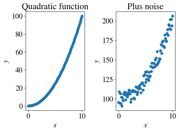
Just like in the previous tutorials, let’s start by generating some artificial ‘measurement’ data. What’s new in this notebook is that we’ll start to consider nonlinear features. To start off simple, first we’ll consider non-linear functions of a single variable (univariate non-linear regression). Let’s try just a quadratic function plus a decent amount of “measurement” noise (and, as before, compute the MSE of this noise in the measurement data):
Code
nr_measurements=100x = np.linspace(0,10,nr_measurements)y = x**2plt.subplot(1,2,1)plt.title('Quadratic function')plt.scatter(x,y)plt.xlabel(r'$x$')plt.ylabel(r'$y$')# Now add some noise:y =100+ y + np.random.uniform(-10,10,x.shape)plt.subplot(1,2,2)plt.title('Plus noise')plt.scatter(x,y)plt.xlabel(r'$x$')plt.ylabel(r'$y$')measurement_error = mean_squared_error(100+x**2 , y)/2print("Measurement error is", round(measurement_error,2))plt.tight_layout()
Measurement error is 14.81
Obviously, fitting these data with a linear function is not going to be a very good model. Let’s try to do so anyway as a first step just for illustrative purposes. More specifically: now that you have learned how a wide range of linear regression models work, we are a bit more justified in being lazy and using one of the very convenient ‘black box’ regression / machine learning functions in scikit-learn. To be precise, the aptly named LinearRegression function, which you used in last week’s lab.
Univariate Linear Regression
One (somewhat cumbersome) implementation detail: LinearRegression expects matrices (rank-2 arrays) as input and wont accept a vector \(x\) or \(y\) like we used before. We can simply turn those into formally matrices but with an ‘empty’ second dimension like this (you can check what \(x\) and \(y\) look like before and after doing this):
Code
print("Shape of x before recasting into array", np.shape(x))x = x[:,None]y = y[:,None]print("Shape of x after recasting into array", np.shape(x))
Shape of x before recasting into array (100,)
Shape of x after recasting into array (100, 1)
You can train the machine learning model, which is really just the fitting stage, by:
As this is not a full-on formal programming class, I’m not going into the logic of the weird python notation LinearRegression().fit(x, y) (and similar syntax below). If you play around with python in general for a while and all the scikit-learn machine learning libraries in particular, you’ll get quite familiar with this notation without having to worry too much about the underlying formal programming concepts. Note that LinearRegression().fit does not need an explicitly defined bias feature \(x_0=1\). I assume it will create that feature internally as part of the function.
Next, your model my_linear_regression_model can make predictions of what the target \(y\) will be for any current or future \(x\) (also with some funny looking python notation). For instance, to see the fitted \(y\) for all our measured \(x\), we use:
Code
y_pred = my_linear_regression_model.predict(x)
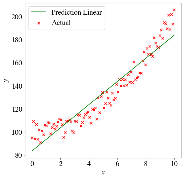
How did we do? Let’s plot the result and compute the error between the fitted \(\tilde{y}\) and measured \(y\):
Code
plt.figure(figsize=(7,7))plt.plot(x,y_pred,color='green',label='Prediction Linear')plt.scatter(x,y,color='red',marker='x', label='Actual')plt.legend(loc='upper left')plt.xlabel(r'$x$')plt.ylabel(r'$y$')error =round(mean_squared_error(y , y_pred)/2,2)print("Regression error over entire data set is", error)
Regression error over entire data set is 48.91
Interestingly, that fit doesn’t look as bad as you might think inside the measurement noise. But of course we know that the relation between the target \(y\) and feature \(x\) should be quadratic, because that is how we generated our artificial data.
So how do we do a non-linear, in this case quadratic, regression?
Univariate Nonlinear Regression
The answers is embarrassingly simple: you just define \(x_1 = x^2\) as the feature (with the superscript 2 an actual quadratic power, to be clear, given all the indices floating around) and then perform a linear regression to fit \(y = \theta_0 + \theta_1 x_1\) with one feature, labeled \(x_1\), which is simply defined as \(x_1 = x^2\).
Again, it may be helpful to think as the measurement data of our features as a spreadsheet. The first column is the bias feature (\(x_1=1\)) and in the second column, we don’t put the measurement data for \(x_1\) itself, but we already take the square of \(x_1\) and define that as our feature. As an example, our measurement data could be pressure, but we define the square of pressure as the input feature for our (linear) regression, with a slope \(\theta_1\).
I myself give this new fitting model the variable name sq_linear_regression_model, but you’ll see that we use the exact same LinearRegression().fit(x1, y) as above.
The model fitting (regression) and then prediction are now just 2 lines of code:
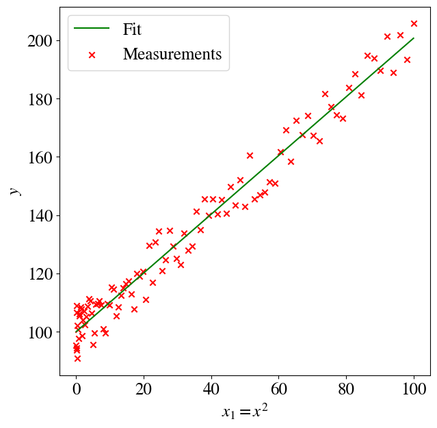
Next, plotting \(y\) versus \(x_1\), the data will indeed look like a linear function. To be very clear, we are not plotting \(y\) versus \(x\) itself, but versus \(x_1=x^2\), the square of our measurements \(x\).
Code
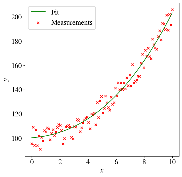
plt.figure(figsize=(7,7))plt.plot(x1,y_pred,color='green',label='Fit')plt.scatter(x1,y,color='red',marker='x', label='Measurements')plt.legend(loc='upper left')plt.xlabel(r'$x_1 = x^2$')plt.ylabel(r'$y$')error =round(mean_squared_error(y , y_pred)/2,2)print("Regression error over entire data set is", error)
Regression error over entire data set is 14.75
We probably want to take a look at the linear fitting coefficients \(\theta_0\) (intercept) and \(\theta_1\) (slope in the above figure). As in last week’s lab, we can pull those out of our fitted sq_linear_regression_model:
Code
theta0 = sq_linear_regression_model.intercept_[0] # the result is given as an array; [0] is the index of the first (and only) elementtheta1 = sq_linear_regression_model.coef_[0][0] # similar to above, the [0][0] only takes the first (and only) element; figured out by just tryingprint("The fitted theta0 and theta1 are: ", round(theta0,2), round(theta1,2))
The fitted theta0 and theta1 are: 100.04 1.01
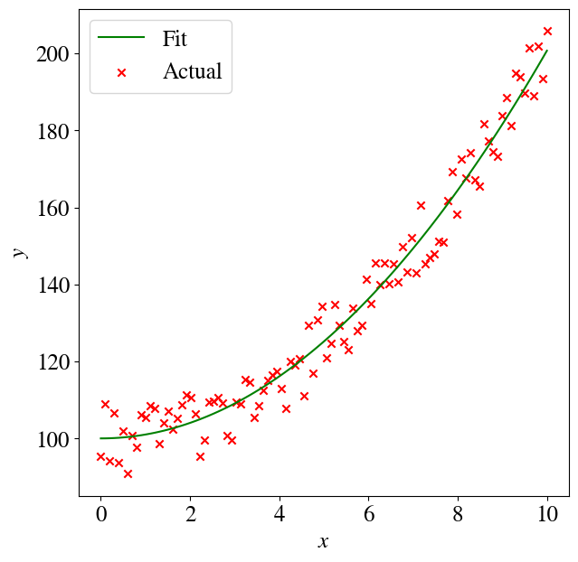
That way we can also go back and plot \(y\) versus \(x\) instead of \(x^2\). In other words \(y = \theta_0 + \theta_1 x^2\):
Code
y_pred = theta0 + theta1*x**2plt.figure(figsize=(7,7))plt.plot(x,y_pred,color='green',label='Fit')plt.scatter(x,y,color='red',marker='x', label='Actual')plt.legend(loc='upper left')plt.xlabel(r'$x$')plt.ylabel(r'$y$')error =round(mean_squared_error(y , y_pred)/2,2)print("Regression error over entire data set is", error)
Regression error over entire data set is 14.75
Multivariate Nonlinear Regression
Now what if we looked at a data-set like the artificial one we created, without knowing exactly what kind of relation it should obey? We could try to fit a higher-order polynomial! For instance: \(y = \theta_0 + \theta_1 x + \theta_2 x^2 + \theta_3 x^3\). All we have to do to generalize the above example is to name/label each higher-order term as an individual feature ( \(x_1 = x\), \(x_2 = x^2\), \(x_3 = x^3\), and of course we can keep going). Again, to avoid confusion, the subscripts label the features while the superscripts are actual powers.
Now we do the linear fitting, and from the \(\theta\)s we can construct our entire polynomial expansion.
Let’s see how it works for this example (starting with a clumsy way of coding each order term = feature individually):
Code
xx = np.zeros([len(x),3])xx[:,0] = x[:,0]xx[:,1] = x[:,0]**2xx[:,2] = x[:,0]**3# Note that 'poly_regression_model' etc are names I give my modelspoly_regression_model = LinearRegression().fit(xx, y)y_pred = poly_regression_model.predict(xx)
Extract the optimal fitted coefficients \(\theta_0 \ldots \theta_3\) and plot the result:
Code
theta0 = poly_regression_model.intercept_[0] # the result is given as an array; [0] is the index of the first (and only) elementtheta1 = poly_regression_model.coef_[0][0] # similar to above, the [0][0] only takes the first (and only) element; figured out by just tryingtheta2 = poly_regression_model.coef_[0][1]theta3 = poly_regression_model.coef_[0][2]y_poly = theta0 + theta1*x + theta2*x**2++ theta3*x**3plt.figure(figsize=(7,7))plt.plot(x,y_pred,color='green',label='Fit')plt.scatter(x,y,color='red',marker='x', label='Measurements')plt.legend(loc='upper left')plt.xlabel(r'$x$')plt.ylabel(r'$y$')print("The fitted theta0 and theta1 are: ", round(theta0,2), round(theta1,2), round(theta2,2), round(theta3,2))error =round(mean_squared_error(y , y_poly)/2,2)print("Regression error for 3rd order polynomial is", error)
The fitted theta0 and theta1 are:  100.3 0.84 0.65 0.03
Regression error for 3rd order polynomial is 14.37
You can see that this worked quite well: the intercept is close to 100, the quadratic term (third one) is close to 1 (because the synthetic data were just \(y=x^2\), and not, say, \(y=5 x^2\)), and the third order term has a very low coefficient.
We do see that there is a non-zero linear term that helps fit the noisy data better (i.e. a somewhat tilted quadratic function), but in comparing the size of each term keep this in mind: the linear feature runs from 0 to 10 while the quadratic term runs from 0 to 100, so for large values of \(x\), say \(x=10\), the contribution from the linear term is \(\theta_1 \times x = -6.8\) while the quadratic term is \(\theta_2 \times x^2 = 115\). In other words, the linear term is a \(<10\)% ‘correction’ to the quadratic one.
We can tidy up this code a little and write it such that it works for any degree polynomial by better vector notation). Let’s go all out and do a 12th order polynomial. First, see how we can generate all the polynomial terms in a basic for loop:
Code
poly_order =12features = np.zeros([len(x),poly_order])for i inrange(poly_order): features[:,i] = x[:,0]**(i+1)
Polynomial fitting parameters are: [ 1.01385163e+02 -1.96624296e+01  3.58192517e+01 -5.07275928e+00
 -2.32640578e+01  2.08232012e+01 -8.76173222e+00  2.20158857e+00
 -3.53474300e-01  3.66508528e-02 -2.37774936e-03  8.78094695e-05
 -1.40892053e-06]
Regression error for 12 order polynomial is 13.61
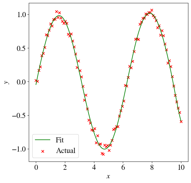
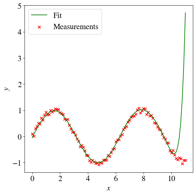
Depending on how much math you’ve taken, you may or may not known/remember that any function can be written as an (theoretically infinite) series of polynomial terms. So the above approach can also fit other nonlinear functions, such as logarithms, exponentials etc. The cell below is just copy-pasted from above, except that we define \(y=\sin(x)\), but fit\(y\) as a polynomial. You can play around with the poly_order to see how many terms of this ‘infinite’ polynomial expansion/series are really needed to fit a sine (7-8 terms already give excellent fitting results).
Polynomial fitting parameters are: [-4.36581431e-02  1.07979444e+00 -1.39852689e-01 -1.14556223e-01
  1.00631022e-01 -1.19216893e-01  6.79001481e-02 -2.09483193e-02
  3.94536619e-03 -4.71331044e-04  3.49615239e-05 -1.46914133e-06
  2.67089478e-08]
Regression error for 12  order polynomial is 0.003
Hopefully you have realized that by moving from linear to nonlinear fitting by introducing higher-order terms as new features, we have also moved from univariate to multivariate regressions. Instead of having higher-order polynomial features \(x_1\), \(x_2\), \(x_n\), we can have any mix of such features, mixed in with completely unrelated features. In other words, we could have features to fit a third-order polynomial in pressure, features that are some power of temperature, and whatever other parameters we may want to consider. Btw, that also includes engineered features like ‘temperature times pressure’ (or some other functional relation).
The only limitation, for our linear regression to work, is that the function is linear in the fitting parameters \(\theta\), so we can fit a model \(y = \theta_1 \sin(x)\) by defining a feature \(x_1 = \sin(x)\), but we cannot use linear regression of fit a model \(y = \sin(\theta x)\) because this is no longer linear in \(\theta\), so we cannot define a feature \(x_1\) such that \(y=\theta_1 x_1\) (ask me if this is not clear).
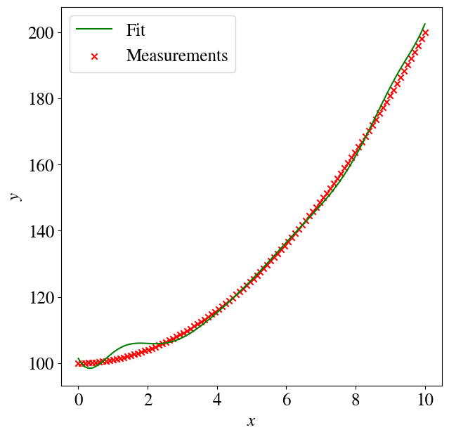
You may also realize that the 12th order polynomial fit to our noisy data fits many more points than a quadratic fit, and thus has a very low error, which could seem like an excellent machine learning result. However, we know that the physical dependence of \(y\) on \(x\) is quadratic (because that’s how we generated the data, but more generally there may be some physical law determining that).
Lingo alert
Basically, using a 12th order polynomial (or 8 or 100 order) is overkill, which in machine learning terminimology (and elsewhere) is referred to as overfitting (or variance). We added more complexity to the model than is warranted by the data. Conversely, in the very top of this notebook, when we fitted just a linear function to these data, we clearly underfitted the data, which is also referred to as bias.
Later, you’ll learn in more detail why this is bad. Essentially, overfitting can better/perfectly match your existing training data but will lead to bad predictions for new data. You’ll then learn how to detect overfitting versus underfitting (or too much variance versus too much bias), and how to ‘fix’ this (through what’s referred to as regularization).
Let’s look at a few preliminary implications of overfitting. First, the 12th order polynomial is not a very good fit to an actual quadratic function without noise:
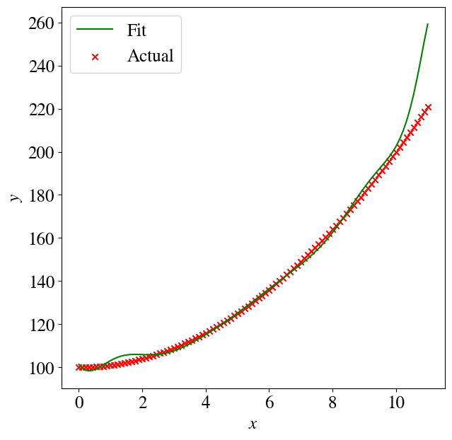
Much much worse, though, are predictions for values outside of the training range (i.e., extrapolation). Let’s see what happens when we repeat almost the exact same code as above, except we use our trained ML model to predict the target \(y\) for values of \(x\) that now run not from 0-10 but over just a slightly wider range of 0-11. You see below that the predictions just ‘explode’ into the wrong direction, which is of course due to the contributions of some very high order terms, like \(x^{12}\) with non-zero coefficients.
Again, in a future session, you’ll learn how to use so-called regularization to reduce this level of overfitting. [Though, not to get everyone’s hopes up, extrapolation outside of a training set range is a major weakness of all machine learning algorithms, even with regularization.]
Multivariate AND Non-linear Regression
So far this week, we have looked at multivariate linear regression, where our hypothesis/model is \(y = \theta_0 + \theta_1 x_1 + \ldots + \theta_1 x_n\), and univariate non-linear regression, which also has a hypothesis/model \(y = \theta_0 + \theta_1 x_1 + \ldots + \theta_1 x_n\) but there each feature was itself defined as a power of a single variable \(x\), i.e. \(x_1 = x\), \(x_2 = x^2\), \(\ldots\), \(x_n = x^n\); all powers of the same independent variable \(x\).
It should be obvious that we can further generalize this to a model that is both non-linear and has multiple measured independent input variables. Let’s choose some variable names for actual physical potential input variables like pressure, \(p\), temperature, \(T\), and, say, salinity, \(s\). We can now define any non-linear multivariate model hypothesis (usually based on some physical knowledge) and our target \(y\) (say, seawater density) could depend on those physical variables through some very complicated function:
\(y = \theta_0 + \theta_1 p + \theta_2 T + \theta_3 s + \theta_4 (p\times T) + \theta_5 s^4 + \theta_6 \log(s/(T\times p)) + \theta 7 \tan(4 p/T) + \ldots\)
by simply defining features (columns in a spreadsheet) \(x_1 = p\), \(x_2 = T\), \(x_3 = s\), \(x_4 = p\times T\), \(x_5 = s^4\), \(x_6 = \log(s/(T\times p)))\), \(x_7 = \tan(4p/T)\), etc. To repeat myself, the only important requirement is that we can write this as a function that is linear in the fitting parameters \(\theta\) that we find with a linear regression model. So we cannot have something as simple as \(y = (\theta_1 x)^2\), because that depends quadratically, not linearly, on the fitting parameter \(\theta_1\).
I won’t give any examples of the above here, partly because visualizations become a bit more difficult with many input features (which would be dimensions of a plot), but you’ll explore this in more detail in the second part of this week’s lab.
Wrap-up Summary, and Next Steps
This week you learned how everything you learned last week for univariate linear numerical regression can be generalized almost trivially to any number of input variabels / features and also to any type of non-linear function, as long as it is linear in the fitting parameters. That means, regular gradient descent, stochastic gradient descent, mini-batch gradient descent, and accelerated methods like (trunctated) Newton method, which uses the second derivative of the Mean Squared Error to set the learning rate.
This means that just 3 weeks into the semester, you already have the Machine Learning tools to efficiently solve a huge range of typical science and engineering problems with ML methods that work for massive amounts of data (unlike the analytical solution methods which, in theory, can be applied to solve the same types of problems).
Next week, you’ll learn how these same methods can again be generalized to, seemlingly, entirely different applications of classification schemes, just be defining a different loss/cost/error function \(J(\theta)\). Such classification is called logistic regression. We’ll follow a similar progression of first looking at logistic linear regression of one variable (univariate), then of multiple variables/features, and then non-linear multivariate logistic regression.