Which platform should I choose?

✏️ After this lecture, try the Practice exercise

Multivariate linear regression

Load various python libraries

First I load a bunch of external libraries. Only a small fraction of the libraries below are actually used in this notebook, but I just use the same ‘preamble’ in all my notebooks so I have access to all the libraries I frequently end up using. If you were to delete all of them, the following error messages in other cells will let you know which libraries to add back in.

from __future__ import division
import numpy as np
import matplotlib.pyplot as plt
# from matplotlib import animation
from IPython import display
import scipy.sparse as sp
import scipy.sparse.linalg
from scipy.linalg import solve_banded
from scipy import optimize

import time
%matplotlib inline
# %matplotlib notebook
from IPython.core.debugger import set_trace
plt.rcParams['figure.dpi'] = 100
# plt.rcParams['text.usetex'] = True
plt.rcParams.update({'font.size': 18, 'font.family': 'STIXGeneral', 'mathtext.fontset': 'stix'})

import pandas as pd

from sklearn.tree import DecisionTreeRegressor
from sklearn.ensemble import RandomForestRegressor

from sklearn.metrics import mean_absolute_error,mean_squared_error
from sklearn.model_selection import train_test_split
# To insert values for missing data
from sklearn.impute import SimpleImputer
# To translate text cell values into numerical labels
from sklearn.preprocessing import LabelEncoder
from sklearn.utils import shuffle
# State of the art Extreme Gradient Booster:
from xgboost import XGBRegressor

from sklearn.linear_model import LinearRegression, Ridge, Lasso
# Plotting of decision trees:
from sklearn.tree import export_graphviz
import IPython, graphviz, re, math

#Neural networks:
#from keras.models import Sequential
#from keras.layers import Dense
#from keras.wrappers.scikit_learn import KerasRegressor
#from keras.callbacks import ModelCheckpoint

from sklearn.model_selection import cross_val_score
from sklearn.model_selection import KFold
from sklearn.preprocessing import StandardScaler
from sklearn.pipeline import Pipeline

from mpl_toolkits.mplot3d import Axes3D  # noqa: F401 unused import



small = 0.0000000001

Generate synthetic data for multi-variate linear regression

Mathematically, in multivariate linear regression we have \(y = \theta_0 + \sum_{j=1}^n \theta_j x_j\) for \(n\) features (independent variables) that we number as \(x_j = x_1, x_2, \ldots, x_n\) with the coefficients (slopes) in the linear model labeled as \(\theta_j = \theta_1, \theta_2, \ldots, \theta_n\). As we increase complexity, we need more and more indices to label stuff, which can be the hardest to keep straight… Remember that we call all features by the generic symbol \(x\), but depending on the problem, these stand for, for example, \(x_1\) is temperature, \(x_2\) is pressure, \(x_3\) is moisture content etc. We then try to predict a single target \(y\) (say adsorption amount) as a function of all the (temperature, pressure, moisture; or \(x_1\), \(x_2\), \(x_3\)) features. For each of those features of course we need many samples or measurements (say, 100 temperatures, 100 presssures etc). In the previous tutorial, we labeled these measurement points as \((x_i, y_i)\). In this notebook, to avoid confusion with the index labeling different features, we will instead use \((x_1^{(i)}, x_2^{(i)}, \ldots, x_n^{(i)}, y^{(i)})\) for a single measurement point \(i\) (for example: the adsorption amount \(y^{10}\) for temperature \(x_1^{10}\), pressure \(x_2^{10}\) and moisture content \(x_3^{10}\)).

Allowing for \(n\) features means that we are working in an \(n\)-dimensional space. Actually, because we also have the intercept \(\theta_0\) and associated auxiliary feature \(x_0=1\) (see previous turorial), we really have a \(n+1\) space. This, in general, makes it a bit hard to visualize anything. For this reason only, this notebook considers only 2 features \(x_1\) and \(x_2\) (and \(\theta_0\), \(\theta_1\), and \(\theta_2\)) to demonstrate, and illustrate, the generalization of univariate to multivariate linear regression (nonlinear regression will be intruduced in the next notebook). The code below can just as easily be applied to any large number \(n>2\) of features, though. When we get to the most complicated machine learning problems of image recognition by neural networks later in the semester, we will use hundreds of features but still apply many of the exact same algorithms as in the notebooks today.

Implementation: the cell below again generates some synthetic data. We start with equidistant points \(0<x^{(1)}<10\) and \(-5<x^{(2)}<5\) (100 each). Next, we generate every combination of the \(x^{(1)}\) and \(x^{(2)}\) points by using the numpy function np.meshgrid again. So we end up with $100 = $ 10,000 measurement points (note that our machine learning algorithms want these as 10,000 element columns, but for plotting it can be useful to have them as \(100\times 100\) matrices, so we save both).

Optional detailed explanation of mesh_grid.

This may be a new concept and as always I recommend testing for yourself in jupyter how this works if you’re not already familiar with this. Later in the semester I will do less of this myself to keep the length of these lecture notes somewhat under control, but for now let me help with a very simple example (pay attention to the comments for meshgrid):

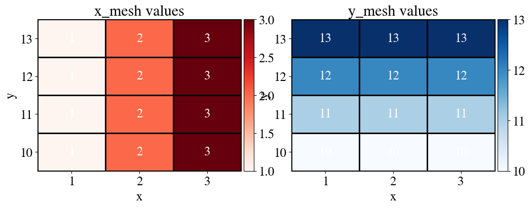
x_values = np.linspace(1,3,3)

print(f"x values are {x_values.astype(int)}.\n")
# Pay attention, the above is a fancier way to make a formatted print statement
# with variables embedded in the text. The simpler unformatted way we used before is:
# print("x values are", x_values, ".")

y_values = np.linspace(10,13,4).T
print(f"y values are {y_values.astype(int)}.\n")

x_mesh, y_mesh = np.meshgrid(x_values, y_values)
# x_mesh: repeats the x coordinates across rows.
# y_mesh: repeats the y coordinates across columns.

print(f"Meshed x-values are: \n{x_mesh}\n\n with shape {np.shape(x_mesh)}.\n.")
print(f"Meshed y-values are: \n{y_mesh}\n\n with shape {np.shape(y_mesh)}.\n")

x values are [1 2 3].

y values are [10 11 12 13].

Meshed x-values are: 
[[1. 2. 3.]
 [1. 2. 3.]
 [1. 2. 3.]
 [1. 2. 3.]]

 with shape (4, 3).
.
Meshed y-values are: 
[[10. 10. 10.]
 [11. 11. 11.]
 [12. 12. 12.]
 [13. 13. 13.]]

 with shape (4, 3).

Notice both are rows = y, cols = x. That’s the row-column convention in NumPy:

First index = row = y

Second index = column = x

This is opposite from the way math books often write (x, y) as if x comes “first.”

In Python arrays, the “first” index is always rows = vertical = y.

Of course it never hurts to try out some matplotlib visualizations of what we’re doing?

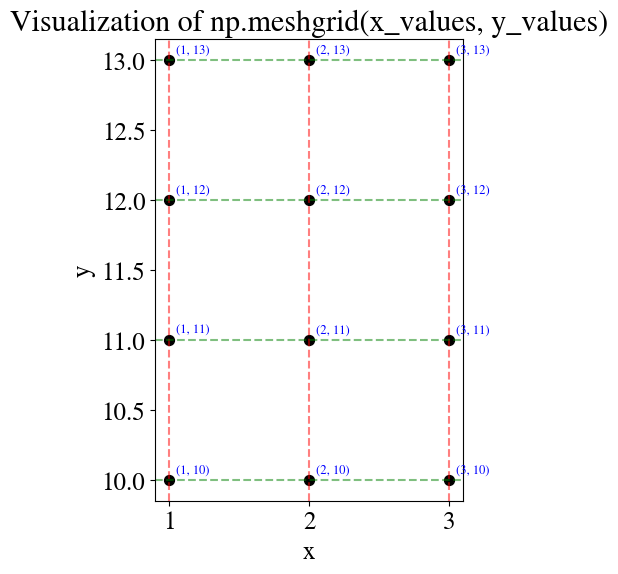
# Plot the meshgrid
fig, ax = plt.subplots(figsize=(6, 6))

# Draw grid points
ax.scatter(x_mesh, y_mesh, c='k', s=50, zorder=2)

# Annotate each point with its (x, y) values
for i in range(x_mesh.shape[0]):
    for j in range(x_mesh.shape[1]):
        ax.text(x_mesh[i, j] + 0.05, y_mesh[i, j] + 0.05,
                f"({int(x_mesh[i, j])}, {int(y_mesh[i, j])})",
                fontsize=9, color="blue")

# Vertical and horizontal grid lines (to emphasize the mesh)
for x in x_values:
    ax.axvline(x, color="red", linestyle="--", alpha=0.5)
for y in y_values:
    ax.axhline(y, color="green", linestyle="--", alpha=0.5)

ax.set_title("Visualization of np.meshgrid(x_values, y_values)")
ax.set_xlabel("x")
ax.set_ylabel("y")
ax.set_aspect("equal")
plt.show()

import matplotlib.pyplot as plt
from mpl_toolkits.axes_grid1 import make_axes_locatable

fig, axes = plt.subplots(1, 2, figsize=(10, 4), constrained_layout=True)

# Left plot: x_mesh values
im1 = axes[0].pcolormesh(x_mesh, y_mesh, x_mesh, cmap="Reds", edgecolors="k", shading="auto")
axes[0].set_title("x_mesh values")
axes[0].set_xlabel("x")
axes[0].set_ylabel("y")

divider1 = make_axes_locatable(axes[0])
cax1 = divider1.append_axes("right", size="5%", pad=0.05)
fig.colorbar(im1, cax=cax1)

# Annotate with values
for i in range(x_mesh.shape[0]):
    for j in range(x_mesh.shape[1]):
        axes[0].text(x_mesh[i, j], y_mesh[i, j], f"{int(x_mesh[i, j])}",
                     ha="center", va="center", color="white")

# Right plot: y_mesh values
im2 = axes[1].pcolormesh(x_mesh, y_mesh, y_mesh, cmap="Blues", edgecolors="k", shading="auto")
axes[1].set_title("y_mesh values")
axes[1].set_xlabel("x")
axes[1].set_ylabel("y")

divider2 = make_axes_locatable(axes[1])
cax2 = divider2.append_axes("right", size="5%", pad=0.05)
fig.colorbar(im2, cax=cax2)

# Annotate with values
for i in range(y_mesh.shape[0]):
    for j in range(y_mesh.shape[1]):
        axes[1].text(x_mesh[i, j], y_mesh[i, j], f"{int(y_mesh[i, j])}",
                     ha="center", va="center", color="white")

plt.show()

Now, we reshape these values into vectors, and then we can also combine them into a matrix/array, and why not add in the bias while we’re at it.

As the last step, we transpose this array (‘turn it sideways’) such that the columns are the features and each row is for a single data point:

m = np.size(x_mesh)
x_vect = x_mesh.reshape(m)
y_vect = y_mesh.reshape(m)
bias = np.ones(m)

print(f"x_vect is: \n{x_vect}\n\n with shape {np.shape(x_vect)}.\n")
print(f"y_vect is: \n{y_vect}\n\n with shape {np.shape(y_vect)}.\n")

x_aug = np.vstack((bias,x_vect,y_vect))
print(f"x_aug is: \n{x_aug}\n\n with shape {np.shape(x_aug)}.\n")

print(f"Machine learning convention is to use features as columns and samples (data points) as rows, \nso we actually need the transpose of this, which is trivial to do with '.T'.")

print(f"x_aug after transpose is: \n{x_aug.T}\n\n with shape {np.shape(x_aug.T)}.\n")

x_vect is: 
[1. 2. 3. 1. 2. 3. 1. 2. 3. 1. 2. 3.]

 with shape (12,).

y_vect is: 
[10. 10. 10. 11. 11. 11. 12. 12. 12. 13. 13. 13.]

 with shape (12,).

x_aug is: 
[[ 1.  1.  1.  1.  1.  1.  1.  1.  1.  1.  1.  1.]
 [ 1.  2.  3.  1.  2.  3.  1.  2.  3.  1.  2.  3.]
 [10. 10. 10. 11. 11. 11. 12. 12. 12. 13. 13. 13.]]

 with shape (3, 12).

Machine learning convention is to use features as columns and samples (data points) as rows, 
so we actually need the transpose of this, which is trivial to do with '.T'.
x_aug after transpose is: 
[[ 1.  1. 10.]
 [ 1.  2. 10.]
 [ 1.  3. 10.]
 [ 1.  1. 11.]
 [ 1.  2. 11.]
 [ 1.  3. 11.]
 [ 1.  1. 12.]
 [ 1.  2. 12.]
 [ 1.  3. 12.]
 [ 1.  1. 13.]
 [ 1.  2. 13.]
 [ 1.  3. 13.]]

 with shape (12, 3).

So now we have a “spreadsheet”-type numpy array which has the bias feature, which is always 1, as the first column, the second column are the values of the \(x_1\) feature and the third column are the values for the \(x_2\) feature, but they are done like two nested loops (our brute force approach) where the outer loop is for \(x_2\) and the inner loop is for \(x_1\), such that for each value of \(x_2\) (in this case, 10, 11, 12, 13), the inner loop runs through all the possible values of \(x_1\) (in this case, 1, 2, 3). Thinking of \(x_1\) and \(x_2\) as, say pressure and temperature (or any other two physical variables you can think of), where “temperature” varies from 1, …, 3 and “pressure” varies from 10, …, 13, we want to have every possible combination of those two ranges. That of course simply defines a 2D grid, or mesh (mesh_grid) of \(x_1\)-\(x_2\) coordinates. With this (perhaps overly) detailed explanation, let’s continue.

Continue with generating synthetic data

We use the same intercept \(\theta_0=100\) and slope \(\theta_1=50\) for the linear dependence on \(x_1\) as before, but now we also have linear dependence with a slope \(\theta_2=12\) in the \(x_2\) direction.

Just to be clear: normally of course we don’t know these \(\theta\) parameters. The purpose of our machine learning algorithms is precisely to find those parameters. We are simply generating fake (synthetic) data, with the additional benefit that we know (by construction) what the ‘true solution’ or outcome of our algorithm should be.

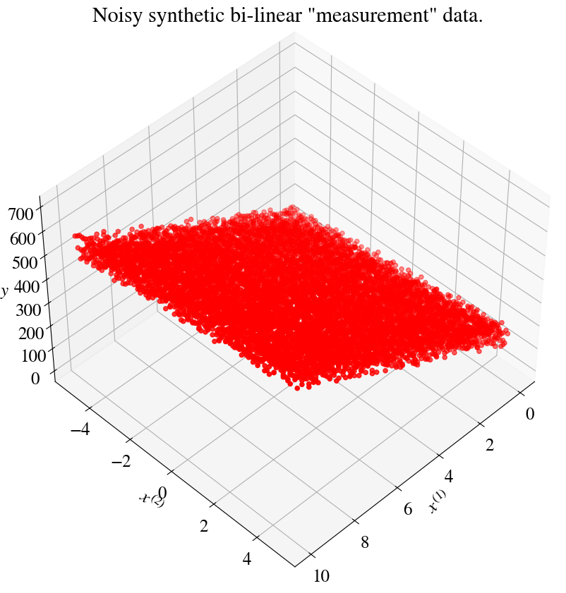
As before, we add some noise to the measurements such that there is no perfect (error-less) fit to a mulitlinear model. In the cell below, you have again the option to add an absolute (abs_noise = True) or relative (abs_noise = False) level of noise.

nr_measurements=100

abs_noise = True

x1_range = np.linspace(0,10,nr_measurements)
x2_range = np.linspace(-5,5,nr_measurements)

x1, x2 = np.meshgrid(x1_range, x2_range)

m = np.size(x1)

############################################################
y_withoutnoise = 100 + 50*x1 + 12*x2

print("Number of x1 and x2 features and targets y:", np.size(x1), np.size(x2), np.size(y_withoutnoise))
############################################################
if abs_noise:
  y = y_withoutnoise + np.random.uniform(-50,50,x1.shape)
else:
  y = y_withoutnoise*(1+ np.random.uniform(-0.1,0.1,x1.shape))

# Save arrays for plotting but also define as 'unrolled' vectors:
x1_m = x1; x2_m = x2 ; y_m = y

x1 = np.reshape(x1,m)
x2 = np.reshape(x2,m)
y = np.reshape(y,m)

Number of x1 and x2 features and targets y: 10000 10000 10000

Let’s plot our synthetic data and compute and print the “experimental error”, which again is just the Mean Squared Error (MSE) of our generated target data plus noise versus the linear functions without noise:

fig = plt.figure(figsize=(10,10))
ax = fig.add_subplot(111, projection='3d')
ax.view_init(45, 45)
ax.scatter(x1, x2, y, c='r', marker='o')

ax.set_title('Noisy synthetic bi-linear "measurement" data.')
ax.set_xlabel(r'$x^{(1)}$')
ax.set_ylabel(r'$x^{(2)}$')
ax.set_zlabel(r'$y$')

measurement_error = mean_squared_error(y_m,y_withoutnoise)/2
print("(Artificial) measurement error is:", round(measurement_error,2))

(Artificial) measurement error is: 418.19

Linear fit with triple loop for slope and two intercepts (brute force)

For this simplest multivariate linear regression problem, with \(n=2\), we have 3 fitting parameters \(\theta_0\), \(\theta_1\), and \(\theta_2\). The ‘stupid’ way to do the fitting is to specify lower and upper limits on each of those parameters and the number of guesses to try within that range. In python (numpy) and also Matlab, you should know how to do this, as for example, theta0 = np.linspace(23,169,100) which will generate 100 equally space numbers between 23 and 169. Alternatively, you may prefer to specify the step-size instead of number of steps, which you can do with theta0 = np.arrange(23,169,10), which generates numbers starting from 23 and incrementing by 10 until it exceeds 169 (the last number in the vector will be as close as you can get below 169).

If any of the new python/numpy functions introduced are not clear, make sure to pop in another code cell and just type in some examples and see what it does! I’ll leave one here as an example.

np.arange(3,100,2.3)

array([ 3. ,  5.3,  7.6,  9.9, 12.2, 14.5, 16.8, 19.1, 21.4, 23.7, 26. ,
       28.3, 30.6, 32.9, 35.2, 37.5, 39.8, 42.1, 44.4, 46.7, 49. , 51.3,
       53.6, 55.9, 58.2, 60.5, 62.8, 65.1, 67.4, 69.7, 72. , 74.3, 76.6,
       78.9, 81.2, 83.5, 85.8, 88.1, 90.4, 92.7, 95. , 97.3, 99.6])

Below, I show 3 different ways to define the values of fitting parameters to try (explicitly typing out the values, by number of steps, and by size of steps). Mostly for illustrative/figure purposes, around 100 values each of \(\theta_1\) and \(\theta_2\) are tried, but only 3 for \(\theta_0\). It would be trivial to also try 100 \(\theta_0\) values, but you can start to see that even for just 3 parameters, that would already require \(100\times 100 \times 100 =\) million (!) loop iterations. For the illustrations below, it will be sufficient to have just 1 or a few \(\theta_0\) values and focus on (plotting the) \(\theta_1\) and \(\theta_2\) dependencies.

[This is just because we only have access to 3 dimensions to plot results, or 4 with some trickery, as you’ll see below. In the previous notebook we had 3D surface plots of the error verus \(\theta_0\) and \(\theta_1\). Here we will plot errors versus \(\theta_1\) and \(\theta_2\), but we can do so for different values of \(\theta_0\). We could just as easily focus on \(\theta_0\) and \(\theta_2\) in plotting, with a fixed (or small number of) \(\theta_1\).]

nrfits1 = 100

theta0 = [30,100,150]
theta1 = np.linspace(2.3,102,nrfits1)
theta2 = np.arange(-1,20,0.2)

nrfits2 = len(theta2)
errors = np.zeros([nrfits2,nrfits1,3])

Do the actual regression with 3 nested loops:

%%time
tries = 0
for k in range(3):
  for j in range(nrfits1):
      for i in range(nrfits2):
          y_pred = theta0[k] + theta1[j]*x1 + theta2[i]*x2
          errors[i,j,k] = mean_squared_error(y_pred , y)/2
          tries = tries+1

CPU times: user 14.6 s, sys: 7.01 ms, total: 14.6 s
Wall time: 14.7 s

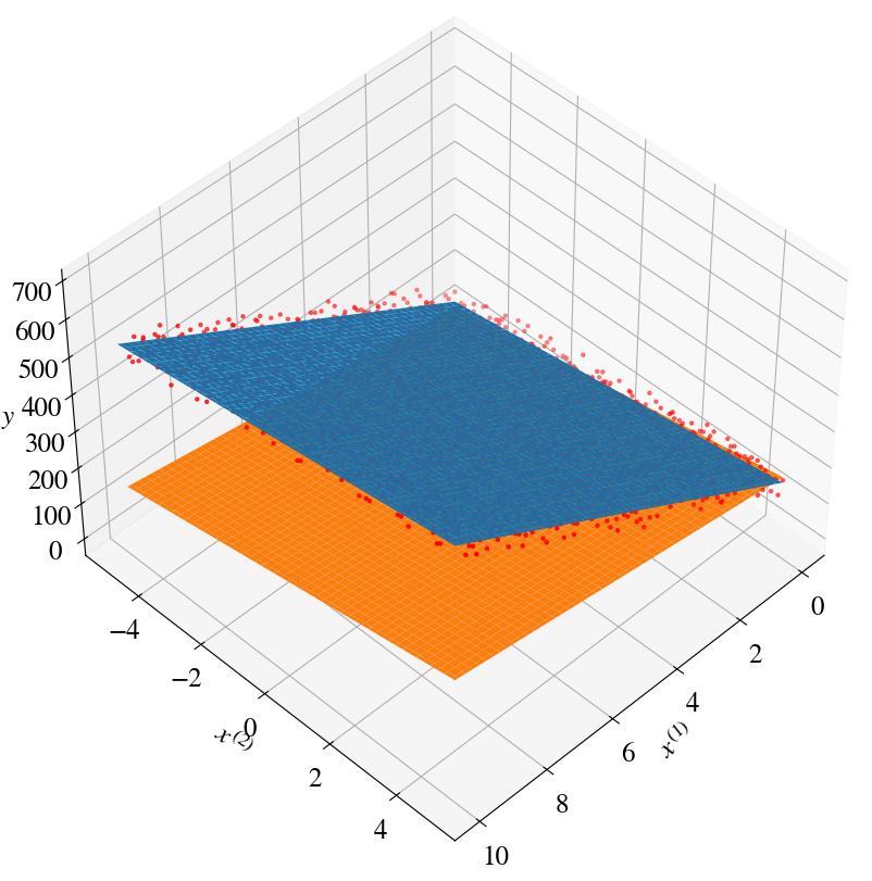
Find the indices of the \(\theta\) values that result in the minimum error (cost) and plot the results. In the previous notebook, the predictions of all (wrong) combinations of \(\theta\)s were plotted as well. Here, just one prediction from a bad fit is plotted for illustrative purposes.

To show how well the fitting worked, the ‘measurement’ points are plotted as well. However, because the fitted plane is hard to see when all 10,000 measurement points are plotted, some more index-wizardy is used to only show every 4th data point.

min_ind = np.where(errors==np.min(errors))

besttheta0 = theta0[min_ind[2][0]]
besttheta1 = theta1[min_ind[1][0]]
besttheta2 = theta2[min_ind[0][0]]

fig = plt.figure(figsize=(10,10))
ax = fig.add_subplot(111, projection='3d')
ax.view_init(45, 45)

print("Plotting only every 4th measurement point, to better visualize the fitted plane")
plot_inds = range(0,len(x1),4)
ax.scatter(x1[plot_inds], x2[plot_inds], y[plot_inds], c='r', marker='.')

# Best fit (note that for this surface plot we used the saved coordinates in array form):
y_pred = besttheta0 + besttheta1*x1_m + besttheta2*x2_m
ax.plot_surface(x1_m, x2_m, y_pred)

# Some arbitrary bad fit for one of our parameter choices:
y_pred = theta0[1] + theta1[10]*x1_m + theta2[80]*x2_m
ax.plot_surface(x1_m, x2_m, y_pred)


ax.set_xlabel(r'$x^{(1)}$')
ax.set_ylabel(r'$x^{(2)}$')
ax.set_zlabel(r'$y$')

print("Minimum fitting/prediction error is:", round(np.min(errors),2), "after trying", tries, "combinations of fitting paramters ")
print("for theta0, theta1, theta2:", round(besttheta0,2), round(besttheta1,2), round(besttheta2,2))

Plotting only every 4th measurement point, to better visualize the fitted plane
Minimum fitting/prediction error is: 421.02 after trying 31500 combinations of fitting paramters 
for theta0, theta1, theta2: 100 49.63 12.0

Error plot

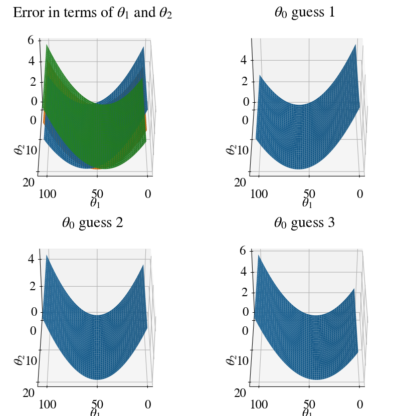
As mentioned above, it already becomes hard to visualize results/algorithms even when we only have 2 features. The error is now a function of 3 variables. Theoretically, this can still be visualized by having 3 axes for \(\theta_0\), \(\theta_1\), and \(\theta_2\) and showing iso-surfaces of the error by different colors, but neither Matlab nor python’s matplotlib have (easy to use) options to plot real 3D data. Instead, we again use surface plots that look like 3D, but are really just 2D: they depend on 2 independent variables \(\theta_1\) and \(\theta_2\) (in this case), while the value of the dependent variable, the error, is shown along the vertical axis.

In other words, the axes are not \(\theta_0\), \(\theta_1\), and \(\theta_2\) but \(\theta_1\), \(\theta_2\), and error. To show the dependence of the error on \(\theta_0\), a different surface is shown for each of its 3 fitted values (the trick to add a 4th dimension).

As a word of caution, matplotlib is also a bit buggy in plotting multiple surfaces in a single plot, and sometimes the surface that appears ‘on top’ should not be there mathematically/physically. For perhaps more clarity, each of the \(\theta_0\) surfaces are plotted in individual plots as well (so 1 combined plot, and 3 individual ones).

fig = plt.figure(figsize=(10,10))
ax = fig.add_subplot(221, projection='3d')
ax.view_init(40, 90)

T1, T2 = np.meshgrid(theta1, theta2)

plt.title('Error in terms of '+r'$\theta_1$' + ' and ' +r'$\theta_2$')

ax.plot_surface(T1, T2, errors[:,:,0]/10000)
ax.plot_surface(T1, T2, errors[:,:,1]/10000)
ax.plot_surface(T1, T2, errors[:,:,2]/10000)

ax.set_xlabel(r'$\theta_1$')
ax.set_ylabel(r'$\theta_2$')

# Repeat panels for individual values of theta0
# First one:
ax = fig.add_subplot(222, projection='3d')
ax.view_init(40, 90)
plt.title(r'$\theta_0$' + ' guess 1')

ax.plot_surface(T1, T2, errors[:,:,0]/10000)

ax.set_xlabel(r'$\theta_1$')
ax.set_ylabel(r'$\theta_2$')

# Second one:
ax = fig.add_subplot(223, projection='3d')
ax.view_init(40, 90)
plt.title(r'$\theta_0$' + ' guess 2')

ax.plot_surface(T1, T2, errors[:,:,1]/10000)

ax.set_xlabel(r'$\theta_1$')
ax.set_ylabel(r'$\theta_2$')

# Third one:
ax = fig.add_subplot(224, projection='3d')
ax.view_init(40, 90)
plt.title(r'$\theta_0$' + ' guess 3')

ax.plot_surface(T1, T2, errors[:,:,2]/10000)

ax.set_xlabel(r'$\theta_1$')
ax.set_ylabel(r'$\theta_2$')

Text(0.5, 0.5, '$\\theta_2$')

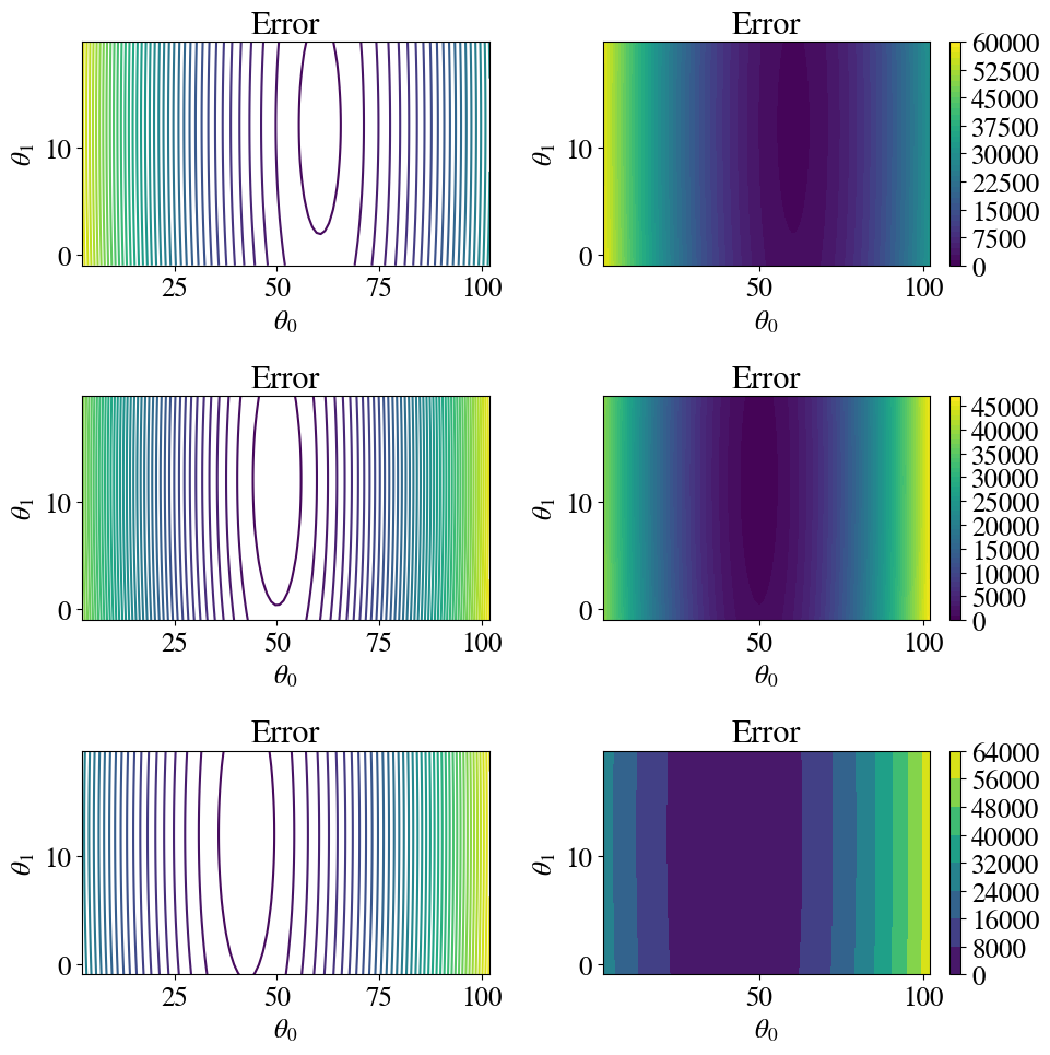
Another way to plot \(z(x,y)\) data is to use coloured or line contour plots. Below, line-contours and colour-filled contours are shown for each of the 3 \(\theta_0\) values.

fig = plt.figure(figsize=(10,10))

plt.subplot(3,2,1)
plt.contour(T1, T2, errors[:,:,0], levels=50)
plt.xlabel(r'$\theta_0$')
plt.ylabel(r'$\theta_1$')
plt.title('Error')


plt.subplot(3,2,2)
plt.contourf(T1, T2, errors[:,:,0], levels=50)
plt.colorbar()

plt.xlabel(r'$\theta_0$')
plt.ylabel(r'$\theta_1$')
plt.title('Error')

#################
plt.subplot(3,2,3)
plt.contour(T1, T2, errors[:,:,1], levels=50)
plt.xlabel(r'$\theta_0$')
plt.ylabel(r'$\theta_1$')
plt.title('Error')


plt.subplot(3,2,4)
plt.contourf(T1, T2, errors[:,:,1], levels=50)
plt.colorbar()

plt.xlabel(r'$\theta_0$')
plt.ylabel(r'$\theta_1$')
plt.title('Error')

plt.subplot(3,2,5)
plt.contour(T1, T2, errors[:,:,2], levels=50)
plt.xlabel(r'$\theta_0$')
plt.ylabel(r'$\theta_1$')
plt.title('Error')


plt.subplot(3,2,6)
plt.contourf(T1, T2, errors[:,:,2], levels=50)
plt.colorbar()

plt.xlabel(r'$\theta_0$')
plt.ylabel(r'$\theta_1$')
plt.title('Error')

plt.tight_layout()

(Vectorized) Gradient Descent Method

The Gradient Descent Method can be generalized to \(n\) features (independent variables \(x_j\)) and written in an efficient notation in which \(x^{(i)}_0 =1\) for all \(i\), as:

• \(\theta_0^\mathrm{new} = \theta_0 - \alpha \frac{\partial J}{\partial \theta_0} =\theta_0 - \frac{\alpha}{m} \sum_{i=1}^m (\theta_0 x_0^{(i)} + \theta_1 x_1^{(i)} + \theta_2 x_2^{(i)} + \ldots + \theta_n x_n^{(i)} - y^{(i)})\times x_0^{(i)}\),
• \(\theta_1^\mathrm{new} = \theta_1 - \alpha \frac{\partial J}{\partial \theta_1} =\theta_1 - \frac{\alpha}{m} \sum_{i=1}^m (\theta_0 x_0^{(i)} + \theta_1 x_1^{(i)} + \theta_2 x_2^{(i)} + \ldots + \theta_n x_n^{(i)} - y^{(i)})\times x_1^{(1)}\).
• \(\ddots\)
• \(\theta_n^\mathrm{new} = \theta_n - \alpha \frac{\partial J}{\partial \theta_n} =\theta_n - \frac{\alpha}{m} \sum_{i=1}^m (\theta_0 x_0^{(i)} + \theta_1 x_1^{(i)} + \theta_2 x_2^{(i)} + \ldots + \theta_n x_n^{(i)} - y^{(i)})\times x_n^{(1)}\).

The notation, and also implementation, is much simpler if we use vector-matrix notation.

Define the \(n+1\) length vector \(\vec{\theta} = (\theta_0, \theta_1, \ldots, \theta_n)\) and similarly vector \(\vec{\theta}^\mathrm{new}\), and the \(m\times (n+1)\) matrix \(X\), which has \(m\) rows for each measurement point and \(n+1\) columns. The first column is the auxiliary feature \(x_0^{(i)}=1\) for all (rows) \(i\) and the other columns are for the \(n\) ‘actual’ features. Think of \(X\) as a spreadsheet with all your data (except the target column \(y\)).

A prediction vector \(\vec{\tilde{y}}\) then follows from our (vector) linear model hypothesis \(\vec{h}(X;\vec{\theta})\) as:

\(\vec{\tilde{y}} = \vec{h}(X;\vec{\theta}) = X \cdot \theta\),

where the \(\cdot\) indicates proper matrix-vector multiplication.

With these definitions, we can simple write (and implement):

\(\vec{\theta}^\mathrm{new} = \vec{\theta} - \frac{\alpha}{m} ((\vec{\tilde{y}}-\vec{y}) \cdot X)\)

As mentioned before, using a for loop does not really make sense. On the one hand we don’t really know how many iterations we need to get an accurate enough fit; on the other hand, if we pick a very large number, we may already reach the most accurate fit early on and do many more iterations for no good reason. In the code below, we therefore use a while loop. We select our own tolerance parameters (as small number) and continue improving our fit until the cost function (error) improves less than that tolerance in a given iteration.

Running this version, you see that out of the 31,500 iterations used above, we only need 476. The code is now 34 times faster than the one we started with.

%%time
nrsteps = 10000

thetas = np.zeros([nrsteps,3])
errorsGD = np.zeros(nrsteps)

alpha = 0.05
alpha_m = alpha/m

x_aug = np.zeros([m,3])
x_aug[:,0] = 1
x_aug[:,1] = x1
x_aug[:,2] = x2

# Initial guess:
thetas[0,:] = [25,10,2]

i=0
converged = False
tolerance = 1e-4
while not converged:

    hypothesis = x_aug.dot(thetas[i,:])

    errorsGD[i] = mean_squared_error(hypothesis,y) /2

    thetas[i+1,:] = thetas[i,:] -  alpha_m * (hypothesis - y).dot(x_aug)

    if np.abs(errorsGD[i]-errorsGD[i-1]) < tolerance:
      converged = True
      print("Converged in", i, "iterations with thetas: ", round(thetas[i+1,0],2),round(thetas[i+1,1],2),round(thetas[i+1,2],2), "and error ", round(errorsGD[i],2))
    i+=1

Converged in 478 iterations with thetas:  101.04 49.89 12.06 and error  417.96
CPU times: user 319 ms, sys: 0 ns, total: 319 ms
Wall time: 336 ms

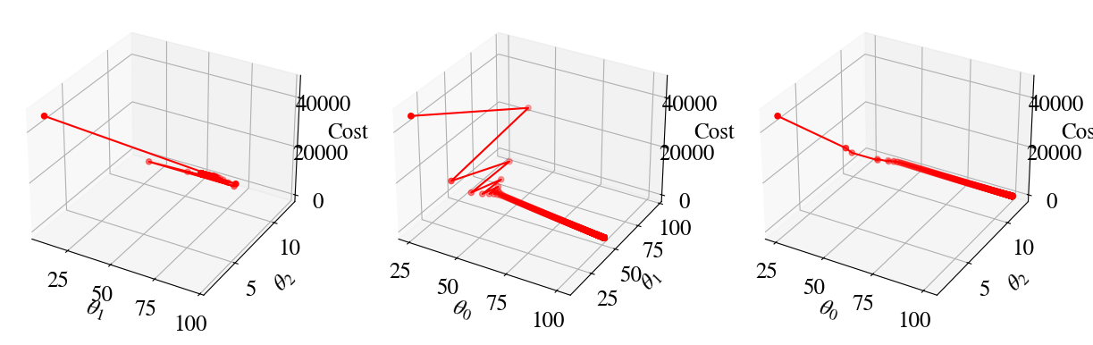
Again the error is a function of 3 \(\theta\) variables now, which is hard to visualize. Below, the error during the gradient descent is plotted in three panels as a function of, respectively, (\(\theta_1\), \(\theta_2\)), (\(\theta_0\), \(\theta_1\)), and (\(\theta_0\), \(\theta_2\)).

thetas_batch = thetas[:i,:]
error_batch = errorsGD[:i]

fig = plt.figure(figsize=(15,5))
ax = fig.add_subplot(131, projection='3d')
ax.set_xlabel(r'$\theta_1$')
ax.set_ylabel(r'$\theta_2$')
ax.set_zlabel('Cost')

TT0 = thetas_batch[:,1]
TT1 = thetas_batch[:,2]

ax.scatter(TT0, TT1, error_batch, c='r', marker='o')
ax.plot(TT0, TT1, error_batch, color='r')

ax = fig.add_subplot(132, projection='3d')
ax.set_xlabel(r'$\theta_0$')
ax.set_ylabel(r'$\theta_1$')
ax.set_zlabel('Cost')

TT0 = thetas_batch[:,0]
TT1 = thetas_batch[:,1]

ax.scatter(TT0, TT1, error_batch, c='r', marker='o')
ax.plot(TT0, TT1, error_batch, color='r')

ax = fig.add_subplot(133, projection='3d')
ax.set_xlabel(r'$\theta_0$')
ax.set_ylabel(r'$\theta_2$')
ax.set_zlabel('Cost')

TT0 = thetas_batch[:,0]
TT1 = thetas_batch[:,2]

ax.scatter(TT0, TT1, error_batch, c='r', marker='o')
ax.plot(TT0, TT1, error_batch, color='r')

Advanced / Accelerated / Higher-Order Regression Methods (e.g., Newton)

To take advantage of the advanced/accelerated methods, we write the functions to compute the cost and cost-gradient in a general form that will apply to any number of (multivariate) features. Notice how elegant these functions are in matrix-vector form! Only 1 line of code for each function.

def cost(theta, x_aug, y):
    return mean_squared_error(x_aug.dot(theta),y) /2

def gradient(theta, x_aug, y):
    return (x_aug.dot(theta) - y).dot(x_aug)/len(y)

def callbackF(theta):
    global Nfeval, x_aug, y,saveresults
    error = cost(theta, x_aug,y) # mean_squared_error(x_aug.dot(theta),y) /2
    print('iter ={0:4d}   theta0 ={1: 3.6f}   theta1 ={2: 3.6f}  theta2 ={3: 3.6f}   error ={4: 3.6f}'.format(Nfeval, theta[0],theta[1],theta[2],error))
    Nfeval += 1

Doing the regression is now as easy as just calling the optimize function, with some initial guess for all \(n\) parameters in \(\vec{\theta}\). To be fully general and not pick a ‘smart’ initial guess, below I start with all \(\theta_j=0\) (coded for any number of features).

%%time
[nr_measurements,nr_features] = np.shape(x_aug)
print("Number of measurements and features (including bias feature x0=1):",nr_measurements,nr_features )
alltheta = np.zeros(nr_features)

Nfeval = 1

result = optimize.minimize(cost, alltheta, args=(x_aug,y), method='TNC', jac=gradient, \
                           options={'disp': True}, callback=callbackF,tol=0.01)

if result.success:
    besttheta = result.x
    nriterations = result.nit
    print("Converged after", result.nit, "iterations to best theta fits:", besttheta)
else:
    print("Accelerated method did not work, maybe try gradient descent.")

y_pred_NM = x_aug.dot(besttheta)
error_NM = mean_squared_error(y_pred_NM,y)/2
print("Error of accelerated method is:", round(error_NM,2))

Number of measurements and features (including bias feature x0=1): 10000 3
iter =   1   theta0 = 1.588261   theta1 = 9.862131  theta2 = 0.464535   error = 52683.187809
iter =   2   theta0 = 1.978227   theta1 = 64.687214  theta2 = 0.589906   error = 2226.626899
iter =   3   theta0 = 5.108684   theta1 = 64.637186  theta2 = 12.740402   error = 1594.896994
iter =   4   theta0 = 15.151902   theta1 = 60.370398  theta2 = 13.037659   error = 1453.392563
iter =   5   theta0 = 101.211910   theta1 = 49.864977  theta2 = 12.059353   error = 417.956781
Converged after 5 iterations to best theta fits: [101.2119101   49.86497702  12.05935344]
Error of accelerated method is: 417.96
CPU times: user 15.1 ms, sys: 0 ns, total: 15.1 ms
Wall time: 18.7 ms

Again, we find an accurate solution in only a few iterations, whereas a fully nested-loop approach might take a million trials! Even when cheating in this case, where we only used 3 guesses for \(\theta_0\) in the nested loops, this last accelerated method is 360 times faster than what we started with in the top.

To be very explicit: the (Accelerated) Gradient Descent Methods are relatively insensitive to the number of features we want to consider. You just saw that we only needed 4-5 iterations for 2 features, while we did 2-3 iterations for a single feature (actually, this method converges for just one step for each feature, plus the initial guess, so n+1 steps/iterations). In contrast, when using nested loops in which \(u\) different guesses are tried for each parameter, a total number of \(u^{n+1}\) iterations are done. Example: in this notebook we considered \(n=2\) features and if we tried \(u=100\) values for each parameter (\(\theta_0\), \(\theta_1\), \(\theta_1\)), we woud need \(100^{2+1} = 100^3\) is a million trials. Now, 100 values for each feature is hardly excessive. If we had 10 features, nested loops would require \(100^{10} = 10^{20}\) iterations. Obviously, even for a lazy coder with nearly infinite computational resources, this aproach is simply not feasible.

This notebook can be short, because once we write the cost (error) and its gradient in vector-matrix form, it really doesn’t matter whether we have 1, 2 or a million diffent features \(x\) to predict our target objective \(y\).

For this week, there is a second separate notebook that generalizes multivariate linear regression to multivariate non-linear regression. Make sure that check out that notebook as well.

---

✏️ Next up: Practice: Multivariate Linear Regression