In this lab, we will go straight to one of the most complicated tasks in Machine Learning: Computer Vision. In particular, you will learn how to automatically classify images into 10 different categories. In other words, our target \(y\) will have 10 different possible labels, 0, 1, 2, …, 9. Actually, these labels happen to be exactly what we are classifying: we’re considering images of hand-written numbers and will try to recognize what those numbers are. As an application, you can think of the US Postal Service scanning mail envelopes and trying to automatically detect the address numbers and zip-codes to send the mail to, rather than manually sorting the mail.
As always, we’ll start by loading some relevant python modules:
Load python modules
Code
from __future__ import divisionimport numpy as npimport matplotlib.pyplot as plt%matplotlib inlineimport timeimport pandas as pdfrom scipy import optimizefrom sklearn.metrics import mean_squared_errorfrom tabulate import tabulateplt.rcParams['figure.dpi'] =100plt.rcParams.update({'font.size': 18, 'font.family': 'STIXGeneral', 'mathtext.fontset': 'stix'})
Load data
Ths lab demonstrates multiclass classification with logistic (linear) regression. A later notebook will model the exact same problem with a neural network, coded from scratch.
The data consist of 5000 pictures of handwritten numbers, which are labeled 0 \(\ldots\) 9 (these are the 10 categories). Each picture is 20x20 pixels and each of the pixels is a ‘feature’ (independent variable \(x_i\)), while \(y\) is the multiclass target.
In summary, we have 5000 labeled datapoints (i.e., this is supervised learning) with 20x20 = 400 features (for each picture sample, plus the bias).
In real applications, like the pictures you take with your smartphone, which likely has (at least) a 12 megapixel camera, each training example (a picture) has 12 million features, so your feature array would already have 5000 x 12 million = 60 billion elements for a linear model and move into the trillions for a polynomial model.
So let’s start with a linear model and low resolution images…
I hosted these data for you and you can import directly into this notebook with similar syntax as in previous labs:
Code
data = pd.read_csv('http://astro.pas.rochester.edu/~moortgat/ex3data1.txt')
As always, you can use .head() and/or .info() to get more information on these data.
Next, we turn the pandas dataframe into a numpy array using the .iloc index notation.
The original data were from Matlab, which doesn’t have a 0 index. The number 0 was mapped to 10. In python we do have the zero index, so we set all values 10 to 0 with the np.where function.
We have 400 features for the 20x20 pixels and we will perform multiclass classification, where the numbers 0 \(\ldots\) 9 represent 10 classes, categories, or labels (num_labels).
Code
y = np.array(data.iloc[:,1])X = np.array(data.iloc[:,2:])# Useful python notation: you can use np.where to search for any# elements in an array that satisfy some condition (such as all negative values,# perhaps any NaN not-a-number values, etc). In this case, when that condition# is true, we change y=10 to y=0, and we leave y as it was otherwose (for all other# elements in the array):y = np.where(y==10, 0, y)num_labels =10print("Dimensions of target y", np.shape(y), "and features X", np.shape(X))
Dimensions of target y (5000,) and features X (5000, 400)
Split into training and validation data
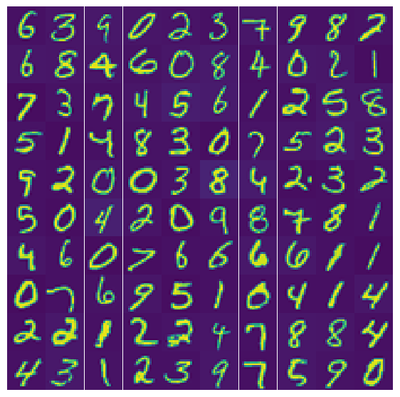
Next, we define a random order of the 5000 indices of the 5000 training data (number of ‘measurements’), and then randomly select 100 of those, i.e. 100 of the 20x20 pixel handwritten number pictures. First, we use these to visualize what our data look like, but then we also drop these 100 cases from our training data, such that we can use this set in the end to validate our trained models.
Code
m = np.shape(y)[0]rand_indices = np.random.permutation(m)selection_x = X[rand_indices[100:200], :]selection_y = y[rand_indices[100:200]]X = np.delete(X,rand_indices[100:200],0)y = np.delete(y,rand_indices[100:200])# Add bias feature:[m, n] = np.shape(X)x = np.append(np.ones([m,1]), X, axis=1)# Dimensions of fitting parameters:all_theta_CG = np.zeros([num_labels, n +1])all_theta = np.zeros([num_labels, n +1])
Visualize data
Now we can visualize what our data look like. For each sample, the features where ‘unrolled’ as one row of all 400 pixels. To visualize, we reshape the features (pixels) back into a 20x20 grid (for each of the 100 selected examples). This array is called x_sq below (square images).
We set up a 10x10 array of plt.subplots and plot one of the samples in each of those 100 figure panels. The ‘true’/supervised labels \(y\) are shown as a simple array of numbers for comparison.
Code
x_sq = np.reshape(selection_x, [100, 20, 20], 'F')nrcols =10nrrows =10fig, axs = plt.subplots(nrrows, nrcols, figsize=(7,7))for i inrange(nrrows):for j inrange(nrcols): image_ij = x_sq[i*nrcols + j]# need to flip this upside down (way data are stored)# numpy has a convenient function for this: np.flipud image_ij = np.flipud(image_ij) axs[i,j].pcolor(image_ij) axs[i,j].set_aspect('equal', 'box') axs[i,j].axis('off')# remove whitespace around subplotsfig.subplots_adjust(wspace=0, hspace=0)# print numerical values of the target ynp.reshape(selection_y, [10,10], 'C')
It is also always a good idea to understand your data, so you could inspect the minimum and maximum values of your features, and look at all features for a single ‘measurement’, which in this case is a single image. Remember, that for each measurement/image, the features are the intensity of each pixel. The above image is in 2 colors, but our data in this case are really just grayscale. Somewhat surprisingly, you can see that some pixels have negative values. Also, the values are floating points that are shown in scientific notation by default. Below, I multiply all values by 1000 (just for illustrative purposes, not for computations), and turn the numbers into integers, so it’s a little easier to see what they look like. The images are \(20\times20\) pixels in size, so the pixel values form a \(20\times 20\) matrix/array.
Remember that our hypothesis for logistic regression (classification) is a sigmoid function, which I’ll refer to as \(g(z)\). This is the key difference with respect to (non-) linear regression in which our hypothesis was a linear model of multiple features \(x\). In vector notation (including bias) the linear hypothesis can be written as: \(h(\mathbf{x}; \mathbf{\theta}) = \mathbf{X}\cdot \mathbf{\theta}\). For logistic regression, we will actually still use similar expressions, but for \(z= \mathbf{X}\cdot \mathbf{\theta}\), which is then ‘passed through’ the highly non-linear sigmoid function \(g(z)\). To be very specific: \[ \tilde{y} = h(x,\theta) = \frac{1}{1+\mathrm{e}^{-
\mathbf{X}\cdot \mathbf{\theta}}}.\]
Define a function for the sigmoid function here and make a plot of what it looks like for, say, \(-10<z<10\). You can copy this, and some of the next steps, from the lecture jupyter notebook, but look at each function carefully to make sure you understand exactly what they do.
Code
# Define sigmoid function and plot it
Cost function for logistic regression
The other big difference as compared to numerical/linear regression is that we use a different error measure, the cost function. For logistic regression we use the cost function (shown here for a single measurement):
\[J(\theta) =
- y \log(h(x,\theta))
-(1-y) \log(1-h(x,\theta)).\]
which is zero when both the prediction/hypothesis \(h(x,\theta\)) and the true value of \(y\) are either \(0\) or \(1\), and blows up to infinity when the hypothesis predicts the wrong label \(y\). The true labels \(y\) are always either 0 or 1, whether we are doing binary classification of multiclass classification using the one-versus-all trick.
Define a python-function for the logistic cost function. The inputs should be fitting parameters \(\theta\), measurements \(x\), and true labels \(y\). The output is a single value for the fitting error (cost). You can look in the lecture notes (the jupyter version) again for how to do this.
Code
# Define python-function to calculate fitting error (cost function)
Gradient of logistic cost function
The only remaining component we need for a logistical regression / cartegorization Machine Learning scheme is the gradient of the cost function, such that we can do gradient descent methods as well as more advanced minimization schemes that also need this gradient. Interestingly and surprisingly, the derivative of the cost function with respect to each \(\theta\), when expressed in terms of the cost function itself, turns out to be exactly the same as for the least-squares error of numerical regression. Schematically: \(\frac{\partial J(\theta)}{\partial \theta} = (g(\theta \cdot x) - y)\cdot x\) (where \(\theta\) is the vector of all fitting parameters and \(x\) is the matrix of all features for all measurement points). In other words, the hypothesis is different, but the gradient as expressed in terms of the hypothesis is exactly as before.
Define a python function that calculates the gradient of the cost function:
Code
# Define gradient of cost function# the inputs are the same as for the cost function itself,# but the output is a vector of error gradients in each theta-direction:
At this point, it is probably a good idea to do a quick test that all is working fine. Generate small arrays for \(\theta\), \(x\), and \(y\) and see that all functions work without, e.g., issues with wrong matrix/vector dimensions or transposes. Here’s some example code to play with, e.g. adding the bias.
Code
# try something along the lines of this:theta_t = np.array([-2, -1, 1, 2])xdum = np.reshape(range(1,16),[5,3],'F')/10X_t = np.append(np.ones([5,1]), xdum,axis=1)y_t = np.ones(5); y_t[1]=0;y_t[3]=0print("Features:\n", X_t)print("Target\n", y_t)print("Cost:\n", np.round(cost_logistic(theta_t, X_t, y_t),2))print("Cost gradients:\n", np.round(grad_logistic(theta_t, X_t, y_t),2))
One-Versus-All Categorization with Conjugant Gradient Minimization
One-Versus-All categorization is the generalization of just having a binary yes/no, 1/0 label to having any number of distinct/discrete categories (and associated labels). The principle is again surprisingly trivial: one simply performs as many binary classifications schemes as one has labels/categories. To give a different example from the one considered here: say we want to categorize pictures into [dog, cat, cow, horse, penguin,pig]. One-versus-all, as the name suggests, first categorizes each picture into whether or not it has a dog (i.e. binary yes/no, 1/0 for yes dog, no dog), then whether or not it has a cat, etc.
In this case, one-versus-all means that we do a loop over the 10 labels for possible handwritten numbers (see below: for c in range(num_labels): ). In the first iteration we see whether the number is yes/no a 0, then whether it is a 1, then 2, until 9.
To do this, we use a nifty python trick. For a given value, say \(c=3\), the python notation y==3 will create a boolean vector of True and False elements, depending on which elements of the vector \(y\) are or are not equal to 3. The trick is to then multiply this resulting vector by a number, in this case 1. In asking to perform this operation, python will turn all False elements into 0 and True elements into 1 to perform the element-wise multiplication. If we started with a target vector with labels between 0 and 9, say for 5 test cases we could have y=[0, 3, 5, 8, 9], then 1*(y==3) would result in [0,1,0,0,0]. This is exactly what we want to do one-versus-all multiclass categorization (i.e. by category-by-category binary logistical regression). As with everything else, make sure to add a code cell and play with the boolean array concept to fully understand it.
Code
# Experiment with boolean operations as described above
To do the regression itself, we again have to minimize our cost function, which is identical to the previous module. Below we demonstrate how to do this with the Conjugant Gradient minimizer, which is extremely efficient and only needs between 9 and 41 iterations to find the best fit \(\theta\) to all 401 features in this case. The speed at which it can solve this problem (about 2 seconds) is quite remarkable.
I will give you some example code of how to do this
Code
%%timefor c inrange(num_labels):print("Finding optimum fitting parameter to predict if pictures are of the number", c) y_binary =1*(y==c) all_theta_CG[c,:] = optimize.fmin_cg(cost_logistic, np.zeros(n+1),fprime=grad_logistic, args=(x,y_binary),gtol=0.001)
Finding optimum fitting parameter to predict if pictures are of the number 0
Optimization terminated successfully.
         Current function value: 0.013122
         Iterations: 19
         Function evaluations: 57
         Gradient evaluations: 57
Finding optimum fitting parameter to predict if pictures are of the number 1
Optimization terminated successfully.
         Current function value: 0.028473
         Iterations: 11
         Function evaluations: 34
         Gradient evaluations: 34
Finding optimum fitting parameter to predict if pictures are of the number 2
Optimization terminated successfully.
         Current function value: 0.065916
         Iterations: 22
         Function evaluations: 60
         Gradient evaluations: 60
Finding optimum fitting parameter to predict if pictures are of the number 3
Optimization terminated successfully.
         Current function value: 0.069375
         Iterations: 20
         Function evaluations: 55
         Gradient evaluations: 55
Finding optimum fitting parameter to predict if pictures are of the number 4
Optimization terminated successfully.
         Current function value: 0.046560
         Iterations: 26
         Function evaluations: 72
         Gradient evaluations: 72
Finding optimum fitting parameter to predict if pictures are of the number 5
Optimization terminated successfully.
         Current function value: 0.072524
         Iterations: 28
         Function evaluations: 69
         Gradient evaluations: 69
Finding optimum fitting parameter to predict if pictures are of the number 6
Optimization terminated successfully.
         Current function value: 0.031556
         Iterations: 16
         Function evaluations: 49
         Gradient evaluations: 49
Finding optimum fitting parameter to predict if pictures are of the number 7
Optimization terminated successfully.
         Current function value: 0.042782
         Iterations: 18
         Function evaluations: 54
         Gradient evaluations: 54
Finding optimum fitting parameter to predict if pictures are of the number 8
Optimization terminated successfully.
         Current function value: 0.080899
         Iterations: 52
         Function evaluations: 129
         Gradient evaluations: 129
Finding optimum fitting parameter to predict if pictures are of the number 9
Optimization terminated successfully.
         Current function value: 0.079954
         Iterations: 40
         Function evaluations: 100
         Gradient evaluations: 100
CPU times: user 5.76 s, sys: 1.16 s, total: 6.92 s
Wall time: 3.76 s
Note that optimize.fmin_cg is not a machine learning tool itself but just a general purpose routine to find the minimum of any function. The machine learning part was to define a suitable cost/error function for fitting parameters. Minimizing that cost function is all there is to this entire image recognition problem. The only difference from binary classification problems, such as those described in the lecture, is that we do this 10 times (for c in range(num_labels):) for 10 different binary targets (1*(y==c)).
Of course now we would like to visualize our results and see how well our trained model will perform on the independent validation images that we set aside. We will do this in the next section of the lab.
Predictions & Validation
So what did we actually compute??
It is easy to get lost in all the math, terminology, and coding, so let me rephrase one more time in words:
For multiclass classification, one uses a one-versus-all approach. Here we have 10 classes/categories for the numbers 0 to 9 (equivalent to images of 10 different species of animals), and a data-set of 5000 images that are labeled by those classes. However, instead of solving one large multiclass ploblem, we solve 10 independent binary classification problems, i.e. in a (outer) loop of 10 iterations.
In the first iteration, we solve a machine learning / fitting problem to see whether or not each picture is a 0, in the next iteration we check for every picture if it is a 1 or not, etc. But let’s stay with the first case where we check for pictures of zeros.
To do this, we take a linear combination of the intensity of each pixel, i.e., our 400 features, with 400 fitting parameters \(\theta\), i.e. \(z= X \cdot\ \!^{(0)}\theta\) (where I use the notation \(\ \!^{(0)}\theta\) to indicate the fitting parameters that only categorize whether pictures is of a “0” or not). Important: as always, we have one set of fitting parameters \(\ \!^{(0)}\theta\) to fit every data point in our feature array \(X\) (plus future measurements). In this case, each row in \(X\) is a picture. When we (vector-) multiply the pixels in one picture with the fitting parameters \(\ \!^{(0)}\theta\), we get one value of \(z\) for each row/picture.
Because this is logistic rather than numerical regression, we now apply the sigmoid function, the yes/no switch, to do our binary classification. What does this mean: for a given picture (row in \(X\)), it the value of $z= X !^{(0)} $ is large, the sigmoid functions is \(\approx 1\), which means “yes, this picture is a zero”. If \(z\ll 0\), the conclusion is “no, this picture is not a zero”. If \(z\) is not that far from zero, we get a probability between 0 and 1 that the picture is 0.
In this first iteration, what we just did is to find a single set of \(\ \!^{(0)}\theta\) that is the most successful in predicting whether each picture is a 0 or not (by matching to the labels, because this is a supervised learning algorithm). ‘Most successful’ meaning that the cost, or error, between predictions of 0 and actual labels of 0 is minimized. In the second iteration, we find another/different set of \(\ \!^{(1)}\theta\) that gives the best predictions of whether a picture is a 1, etc. In the end, we find an array/matrix of dimensions \(10\times 400\) values of \(\theta\) fitting parameters.
When we multiply our entire feature array with this large (\(10\times 400\)) matrix of fitting parameters \(\theta\), we get another array: for each picture, i.e. each of 5000 or so rows in our feature array, we get 10 predictions of the probability that that picture is a 0, 1, \(\ldots\), 9 (so for 5000 pictures, \(X\cdot \theta\) is a 5000 \(\times\) 10 array).
The last step therefore is to pick the highest probability for each picture to predict which of the multiple classes/categories it belongs to.
Those last steps are done below:
Have a look at the size of our array of fitting parameters \(\theta\) (whatever you called that variable). It should be \(10\times 401\): 400 pixels plus the bias/intercept of the fit for each category:
Code
# check size of fitting parameter variable
Our formal hypothesis should give 10 probabilities for each picture:
Let’s just have a look at what these look like. I draw a random selection of 10 pictures (i.e. different every time you run this cell) and look at the corresponding hypothesis that we compute above. The results are plotted in a nice table.
For each of the 10 pictures, a row in that table gives the probabilities that that picture was a 0, 1, \(\ldots\), 9. Depending on your draw, you can see that for some pictures one of the probabilities is almost 1, so our algorithm could easily categorize the number. For some other rows/pictures, all the probabilities are pretty low and we just have to pick the highest one and ‘hope for the best’.
The three print statements below the table are 1. Our final prediction based on the maximum probability, using np.argmax, which gives the index of where the maximum number was found; in our problem this is conveniently equal to our actual target of 0, …, 9. If we were matching cats and dogs we’d have to have one more line of code to match the indices to animals. 2. The actual label. If you run the cell a few times, most of the times the predictions and actual labels agree well, and for every row one of the probabilities is close to 1. But every now and then you’ll catch a problem case. 3. A true/false comparison between prediction and actual label.
Code
# Let's just look at first 10 images:ten_random_indices = np.random.permutation(4900)[:10]# For each picture, these are 10 probabilities for each number:y_prob = np.round(hypothesis[ten_random_indices,:],3)# This will pick which probability is highest, and thus our final prediction:y_pred = np.argmax(hypothesis[ten_random_indices],axis=1)# To show a nice table of these probabilities:headers = ["# 0 ","# 1", "# 2", "# 3","# 4", "# 5", "# 6","# 7", "# 8", "# 9"]table = tabulate(y_prob, headers, tablefmt="fancy_grid")print("Probabilities for first 10 images:\n")print(table)print("Maximum probabilities for first 10 images:\n", y_pred)print("Labels ('true' values for first 10 images:\n",y[ten_random_indices])print("Correct predictions:\n", y_pred==y[ten_random_indices])
We can also just do this for the entire dataset at once with one simple statement:
Code
p = np.argmax(hypothesis,axis=1)
To see how well our multiclass categorization algorithm performed for the full problem, we use the same trick as above. The boolean statement p == y will create a vector with True for every correctly identified picture and False for every incorrectly identified pictures. Multiplying by 100 turns True into 100 and False into 0, so if we take the mean/average of the resulting vector, we immediately find the success rate of our full algorithm. (Alternatively, of course we could just do some kind of loop of checking each picture, but the trick below is more efficient.)
Code
accuracy = np.round(np.mean(100*(p == y)),1)print("The accuracy of our machine learning algorithm using Gradient Descent is", accuracy, "%.")
The accuracy of our machine learning algorithm using Gradient Descent is 93.5 %.
(Cross-)validation
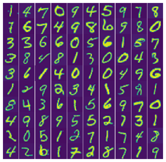
Above, we only checked how well our algorithm performed on our training data. But as you learned in our previous lectures and labs, this can be (sometimes highly) misleading. To see the true accuracy, we need to test its performance on data the algorithm has not seen before. Fortunately, we already ‘set aside’ a set of 100 picture for that purpose. Below, we take those picture and create a feature array that includes the bias ( \(x_0=1\) ) feature. We then multiply by the fitting parameters from our training set to find the probabilities that our validation pictures are a 0, 1, … , 9 and pick the highest probability, just as above. As another way of visualizing, I show a 10×10 array of the predicted numbers for our 100 validation pictures, then a 10×10 array of the ‘true’ labels for the same 100 pictures, and just so you don’t have to compare those two one-by-one, I print a 3rd array with values 1 when the prediction was correct and 0 when it was wrong. For convenience, I also show the actual pictures again; the same set that was already shown at the start of this notebook.
You should see that we achieved a classification accuracy of >90% (depending on what random selections we used). This is pretty remarkable given the challenge of the problem (recognizing wildly varying handwritten numbers from images) and the fact that we still only used linear logistic regress.
Exercise: implement Gradient Descent from scratch!
In the previous sections, I tried to guide you to quickly obtain some actual logistic regression, i.e. classification, results for an interesting problem without getting too bogged down in potential python pitfalls, and providing some codes for nice visualizations of those results. Essentially, you only need to define 3 functions to define our new hypothesis, cost function, and cost gradient.
Assuming this went smoothly, you may have time for a more hands-on practice exercise. Specifically, to avoid using black box sklearn or other optimization routines altogether, and code the logistic regression ‘from scratch’ using standard Gradient Descent to understand even better how this works. Just as for the accelerated method used above, you can use any version of the numerical regression with gradient descent, simply by changing the hypothesis, cost, and cost gradient functions. The best choice is probably the vectorized implementation with a while loop that checks when our errors (cost) have converged and no longer change appreciably in further iterations (by a user-defined accuracy tolerance).
In other words, you can copy that code from a previous lecture/lab (and the lectures notes jupyter notebook for this week) and make suitable changes for logistic regression. If you get the gradient descent to work, you could make your code even fancier by defining the gradient descent as a python function that takes features \(x\) and targets \(y\) as inputs and returns the best fitting parameters \(\theta\) as output. Something like
You could also add additional input arguments to this function, such as the learning rate. This would allow you to easily run gradient descent several times with different learning rates to see which choice performs the best in terms of accuracy and efficiency. You can also choose whether you only want to output the final optimized fitting parameters \(\theta\) or perhaps you want to output the fitting parameters at each iteration to see how they improve, or also output the errors so you can plot the learning curve (error as a function of nr of iterations). I leave this up to your own creativity.
Make sure to always double check the shapes of all your variables, whether or not you need to add a bias column, how to initialize your fitting parameters \(\theta\) with a first initial guess (perhaps just all zeros), etc.
We will build on this work in future labs so it can be helpful to write tidy recyclable codes/functions.
Code
# Implement gradient descent yourself
Conclusions
This week you have learned how we can take the Machine Learning tools developed for numerical (linear and non-linear) regression and use those same tools for the seemingly quite different application of classification schemes.
Specifically, we can apply the same gradient/stochastic/mini-batch gradient descent methods, and their accelerated optimizations, by making only 3 minor modifications:
We use a different model hypothesis by using a sigmoid function that asymptotes to 0 or 1 for small/large values of its argument,
We use a different error metric (cost function) to test whether predictions are good or bad, with a very large (formally infinite) error for wrong predictions,
The gradient of that new cost function can be expressed in terms of the cost function itself in exactly the same way as for the mean-squared-error used in numerical regression.
In the lecture, you also learned how 1. the argument of the sigmoid function \(z=\mathbf{X}\cdot \mathbf{\theta}=0\) defines the decision boundary between predictions of 0 and 1 for given features \(x\), and 2. how we can generalize binary logistic regression to multi-class classification by using a one-versus-all approach in which we only predict one class at a time and loop over all the classes of interest.
In this lab, we went straight to one of the more challenging Machine Learning applications: Computer Vision. In particular, you developed your own object classification algorithms to classify images into 10 different categories, as an illustration of how similar algorithms work that, e.g., Facebook, Google, Amazon and other big data companies use. In such schemes, each image can be considered as a ‘measurement’ and each pixel is a ‘features’, so you can see how these problems can quickly become ‘Big Data’ problems, for which one might want to use memory efficient methods like stochastic gradient descent (fitting only one image at a time).