Artificial Neural Networks for Multi-Class Classification Problems
This notebook accompanies the lecture on Artificial Neural Networks and implements an example to classify images of handwritten numbers. Much of this is based on the famous AI course by Andrew Ng at Stanford and if you want to dig in deeper you can readily watch those lectures on youtube, where you will recognize many of these materials. Those current links are
Ths module demonstrates multiclass classification with an Artificial Neural Network (ANN).
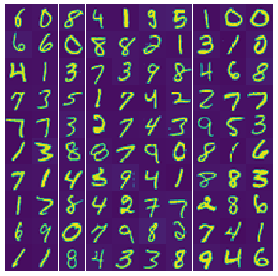
As before, the data consist of 5000 pictures of handwritten numbers, which are labeled 0 \(\ldots\) 9 (these are the 10 categories). Each picture is 20x20 pixels and each of the pixels is a ‘feature’ (independent variable \(x_i\)), while \(y\) is the multiclass target.
Load libraries
Cleaned up a bit to only load necessary libraries.
Code
from __future__ import divisionimport numpy as npimport matplotlib.pyplot as plt%matplotlib inlineimport timeimport pandas as pdfrom scipy import optimizefrom sklearn.metrics import mean_squared_errorfrom tabulate import tabulatefrom progressbar import ProgressBar
Parameters to make figures look nicer:
Code
# Change some default figure properties to make them prettier:plt.rcParams['figure.dpi'] =100plt.rcParams.update({'font.size': 18, 'font.family': 'STIXGeneral', 'mathtext.fontset': 'stix'})plt.rcParams['figure.figsize'] =7,5plt.rcParams['axes.spines.top'] =Falseplt.rcParams['axes.spines.right'] =Falseplt.rcParams['axes.linewidth'] =2plt.rcParams['lines.linewidth'] =3
Generate data
Load data for the 5000 images and construct feature array \(x\) and targets \(y\).
The sigmoid function (\(\frac{1}{1+\mathrm{e}^{-z}}\)) was already defined. We will also need its derivative, which can be written in terms of the sigmoid itself.
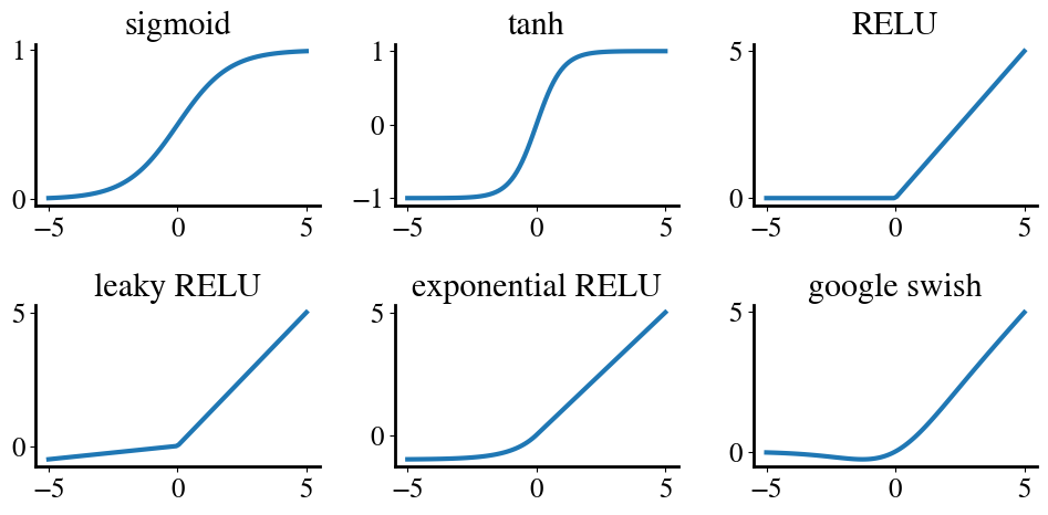
There are a number of other functions, such as the hyperbolic tangent, that basically turn a continuous variable into binary categories (sometimes labeled as 0 and 1, sometimes as -1 and 1, and sometimes as 0 or -1 for an argument \(x<0\) and inceasinly large for \(x>0\)) with some transition in between. In ML lingo, these are called activation functions. In neural networks, in particular, (presented below) sometimes activation functions other than the sigmoid have better performance.
Below we define functions sigmoid and their derivatives d_sigmoid that are already generalized to allow for any activation function that I could find in the literature on ML and neural networks in particular, for future use.
These different activation functions are provided to give you a throrough overview of different ANN approaches, but the familiar sigmoid function is a perfectly fine choice for anything discussed here.
Here’s a simple visualization of what all these activation functions look like, such as the various ‘rectified linear units (RELU link text)’ functions.
I will not discuss the philosophy behind articifial neural networks, inspired by the functioning of the human brain, or some of the technical aspects in full detail here. A number of videos are provided to help with that.
In practical terms, a (artificial) neural network is similar to the logistic regression discussed before. Basically, a ANN just does the same thing twice, or more. As an example, we will consider a shallow artifical neural network with one ‘hidden layer’, which in a sense just means we do logistic regression twice. A deep neural network has multiple hidden layers, which effectively means it does logistic regression multiple times.
Let me explain:
In the logistic regression you have seen before, we have, say, 401 features, we take a linear combination of those with fitting parameters \(\theta\) (\(z = X \cdot \theta\)), and then apply a sigmoid function to the outcome (\(y = g(z)\), the activation function) to determine the probability of a sample/picture/measurement belonging to category 0 or 1 (or any number of categories when doing one-versus-all).
In a shallow neural network (with 1 hidden layer), we try multiple linear combinations of the features with multiple sets of \(\theta\) (this is the first layer); then we apply the sigmoid function to each of those linear combinations, and construct a second linear combination of those sigmoids with an independent set of fitting parameters \(\theta\) to come up with a single final prediction for \(y\).
The basic strength of this approach is that instead of a linear combination of the feature, we have a linear combination of sigmoids of linear combinations of features (… are you still with me?). By introducing those sigmoid in the intermediate step (the hidden layer), the final prediction is actually a highly non-linear model. As you have seen before, non-linear models like high-order polynomials can fit much more complex data, and the same is true for these neural networks (which are not polynomials, but linear combinations of sigmoids).
A different way of thinking about this is that the first layer, which takes many different combinations of your input features, can learn/engineer new features, and then the second layer just performs a regular logistic regression on those new features.
To be a more specific: * In the example below we use an ‘input layer’, which are simply our features (input_layer_size = 400 below), which in an ANN are also called (input) nodes. * The new thing the ANN adds is another layer, the hidden layer, which can be any size we choose; in the example below we choose hidden_layer_size = 25 nodes. * The output from the hidden layer is mapped (by a linear combination) to the ‘output layer’, which is either a single node for a binary classification scheme, or 10 nodes for our multiclass problem here (num_labels = 10).
In a neural network, there is a bunch more bookkeeping, but conceptually it is not as complicated as all the aforementioned may make it sound.
Consider a single picture (or datapoint/measurement in general) with our 400 pixels/features. In a regular logistic regression, we would
Add our bias feature to make a feature array \(X\). Note that for a single picture, this is actually just one row and thus just a vector \(X\).
Take some initial guess of a vector of 401 fitting parameters \(\theta\) and compute \(z = X \cdot \theta\). For a single picture, this is just a single number (the dot product of the vectors \(X\) and \(\theta\)).
For numerical regression, this would be the final prediction, but for logistic regression we take the sigmoid of this one number, which is our hypothesis \(h=g(z)\), as our prediction. For binary categorization, \(h\) would be between 0 and 1 and would postprocess to, say, \(y=1\) if \(h \ge 0.5\) and \(y = 0\) for \(h < 0.5\). You’ve seen how to generalize this in one-vs-all for multiclass problems.
We define a cost/error function between the predicted \(y\) and actual labels, as well as its derivative, and minimize the cost as a function of the fitting parameters \(\theta\). The \(\theta\) that give the lowest prediction error essentially define our ML model.
We do more or less the same for our artificial neural network, again looking at just one picture, in this way: 1. We start with the same feature array \(X^{[1]}\). 2. We multiply not with a 401-element vector \(\theta\) but now by a \(25\times 401\)array of fitting parameters \(\Theta^{[1]}\) (where I will use the new superscript \(^{[1]}\) to denote the first layer). This is the same as taking 25 dot-products with different choices of \(\theta\), each of which is a column in the array \(\Theta^{[1]}\), and thus provides 25 different values for \(\mathbf{z}^{[2]} = X^{[1]} \cdot \Theta^{[1]}\), corresponding to the 25 nodes of this hidden layer. 3. Just like in regular logistic regression, we apply the sigmoid function, but to each node in this layer \(h^{[2]} = g( \mathbf{z}^{[2]})\), so the \(h^{[2]}\) in the hidden layer are 25 hypotheses (= predictions) for 25 different guesses/trials of fitting parameters. 4. This is where the magic kind of happens: we treat the predictions \(h^{[2]}\) (plus a bias) as new features to make a feature array \(X^{[2]}\), take another linear combination of those 25 predictions \(\mathbf{z}^{[3]} = X^{[2]} \cdot \Theta^{[2]}\), and apply the sigmoid function again to end up with our hypotheses for the output layer \(h^{[3]} = g( \mathbf{z}^{[3]})\). 5. For a binary classification problem with only only output node (one final predicted number) \(\Theta^{[2]}\) would just be a vector with length 25+1, the number of hidden nodes plus bias feature. For a multiclass problem, such as the 10 numbers considered here, we can do all classes at once with an \(10\times 26\) array of fitting parameters for the 10 output nodes. In that case, modern implementations usually use the softmax function for the final output instead of sigmoid functions.
ReLU vs Leaky ReLU vs ELU
Cost function
The cost/error of a binary prediction from our neural network is defined exactly the same as for logistical regression. For a single measurement:
\(J(\theta) =
- y \log(h(x,\theta))
-(1-y) \log(1-h(x,\theta)),\)
except that it needs to be evaluated for the hypotheses \(h^{[3]}\) from the output layer. For a multiclass problem, we don’t do one-versus-all, but automatically consider all classes at once. Specifically, the labels for each image –in our image classification problem– are defined as vectors \(y = [0,0,1,0,0,0,0,0,0,0]\) when the image is of a ‘2’, etc. The hypothesis for each node in the output layer is a (pseudo-) probability, so the output would look something like \(h(x,\theta) = [0.01, -0.02, 0.90, 0.4, ..., -0.01]\), and the errors/costs for the 10 categories would be summed to obtain the total error (and also summed over all images/‘measurements’).
As you should know by now, defining the cost function is the key to any machine learning algorithm.
Below we define it for any shallow network (i.e., you can also run it for more or fewer hidden nodes). The inputs are the size of the input layer (nr of features), hidden layer, and output layer (which is the number of labels), the actual features (pixels) \(X\), labels \(y\), and one giant vector of fitting parameters theta. The latter contains both \(\Theta^{[1]}\) and \(\Theta^{[2]}\) sequentially because a general-purpose minimization scheme, like gradient descent, conjugate gradient, Newton etc, don’t care that these are parameters for different layers in an ANN; for a minimization scheme, these are just a long list of numbers to minimize. Turning rank-2 (two-dimensional) arrays \(\Theta^{[1]}\) and \(\Theta^{[2]}\) into one long vector is called unrolling.
Finally, we also Ridge regularize the scheme by adding the summed squares of all fitting parameters \(\Theta^{[1]}\) and \(\Theta^{[2]}\).
The function is obviously a bit longer than before, but not that complicated if you look carefully. The first 15 lines is just setting up arrays with the right dimensions. Line 19 and 22 are exactly the logistical regression from the last module, using \(\Theta^{[1]}\), and lines 22, 23, 25 just do the same thing one more time, essentially, but now with \(\Theta^{[2]}\). Finally, line 30 is the same cost as before, but we had to go through the other steps to get the hypothesis for the output layer. These steps are called ‘forward propagation’ in neural networks (going through all the aforementioned steps from left-to-right if you drew out the network).
First, we define a function that does the ‘forward pass’, which means computing our final hypothesis \(y\), given inputs \(X\), and two arrays of fitting parameters / weights \(\Theta^[1]\) and \(\Theta^[2]\) for the first and second layer of our neural network. Lines 10-15 below just pull these arrays from one long list of \(\theta\) values and reshape them into the appropriate array dimensions. Lines 18-20 are for the first layer and lines 21-23 for the second layer of our ANN.
Code
# --------------------------------------------------------# Forward propagation# --------------------------------------------------------def nn_forward(theta, input_layer_size, hidden_layer_size, num_labels, X):"""Forward pass through a 2-layer neural network. Shapes chosen so that no .T transposes are needed.""" m, n = X.shape# Reshape Thetas for left-to-right matrix flow Theta1_dims = (input_layer_size +1, hidden_layer_size) Theta1_len = np.prod(Theta1_dims) Theta2_dims = (hidden_layer_size +1, num_labels) Theta1 = theta[:Theta1_len].reshape(Theta1_dims) Theta2 = theta[Theta1_len:].reshape(Theta2_dims)# Forward pass X1 = np.c_[np.ones((m, 1)), X] # add bias column (np.c_ is short for np.concatenate) Z2 = X1 @ Theta1 # (m, hidden_layer_size) A2 = sigmoid(Z2) A2 = np.c_[np.ones((m, 1)), A2] # add bias column Z3 = A2 @ Theta2 # (m, num_labels) H3 = sigmoid(Z3) # final output activationsreturn H3, Theta1, Theta2
Before we define our cost function, let me explain an elegant python trick to do the one-hot-encoding when we want to predict multiple classes.
In multiclass classification, we often need to represent each class label as a one-hot vector —
a row of zeros with a single 1 marking the true class.
For example, suppose our dataset has 4 samples and 3 possible classes (num_labels = 3):
if the labels are y = [2, 0, 1, 2], the one-hot encoding should be:
Sample
Label
One-Hot Vector
1
2
[0, 0, 1]
2
0
[1, 0, 0]
3
1
[0, 1, 0]
4
2
[0, 0, 1]
We can create this efficiently in NumPy without loops:
np.zeros((m, num_labels)) → make an all-zero matrix
np.arange(m) → make a list of row indices [0, 1, 2, ..., m-1]
Y[np.arange(m), y] = 1 → set the position (row i, column y[i]) to 1 for each sample
This results in a fully vectorized, fast one-hot encoding operation.
With our definition of our new ANN hypothesis, and the one-hot-encoding of our target labels, we can use the same logistic cost function + Ridge regularization as before:
Code
# --------------------------------------------------------# Cost function with regularization# --------------------------------------------------------def nn_cost(theta, input_layer_size, hidden_layer_size, num_labels, X, y, lambda_r):"""Compute the cost J(Θ) for a 2-layer neural network.""" m = X.shape[0] H3, Theta1, Theta2 = nn_forward(theta, input_layer_size, hidden_layer_size, num_labels, X)# One-hot encode labels Y = np.zeros((m, num_labels)) Y[np.arange(m), y] =1# --- Core cost (cross-entropy) --- eps =1e-12 J =-np.sum(Y * np.log(H3 + eps) + (1- Y) * np.log(1- H3 + eps)) / m# --- Regularization (ignore bias columns) ---# Strip the first column (bias weights) reg = (np.sum(Theta1[1:, :]**2) + np.sum(Theta2[1:, :]**2)) * lambda_r / (2*m) J += regreturn J
Cost gradient
Of course the other ingredient that we need for most solution schemes is the gradient of our cost function, which are the partial derivatives of the cost with respect to each fitting parameter. This may seem daunting when considering the beast of a cost function above, and many think it is, but -certainly in terms of implementation- it is actually not that hard. Without going into too much detail (which is provided in the videos), it essentially builds up the derivatives by the familiar chain rule. This effectively means starting from the right (the output layer) and working back to the left, which is why this step is called the back propagation, or even more slangly, back prop.
In the long-looking code below, the first 26 lines are actually the same as in the cost function, while the back prop itself is only a few short lines between lines 29 and 36. In line 31, d3ij[:,k] simply takes the difference between our final/output prediction/hypothesis for each label \(k\) versus the true label \(y\). Line 33 shows the whole chain rule. Lines 42-45 just stick all the fitting parameters back into a single long vector/list in the right order. For more details on the back-prop, watch the video.
Code
def nn_gradient(theta, input_layer_size, hidden_layer_size, num_labels, X, y, lambda_r):""" Compute backpropagation gradients for a 2-layer neural network using the same conventions as nn_forward (no transposes in the forward pass). Shapes: Theta1: (input_layer_size + 1, hidden_layer_size) Theta2: (hidden_layer_size + 1, num_labels) X: (m, input_layer_size) """ m = X.shape[0]# Forward pass H3, Theta1, Theta2 = nn_forward(theta, input_layer_size, hidden_layer_size, num_labels, X)# Recompute intermediates needed for backprop X1 = np.c_[np.ones((m, 1)), X] # (m, input+1) Z2 = X1 @ Theta1 # (m, hidden) A2_no_bias = sigmoid(Z2) # (m, hidden) A2 = np.c_[np.ones((m, 1)), A2_no_bias] # (m, hidden+1)# One-hot encode labels Y = np.zeros((m, num_labels)) Y[np.arange(m), y] =1# Error in output layer d3 = H3 - Y # (m, num_labels)# Error in hidden layer (excluding bias) d2 = (d3 @ Theta2[1:, :].T) * (A2_no_bias * (1- A2_no_bias)) # (m, hidden)# Unregularized gradients Theta2_grad = (A2.T @ d3) / m # (hidden+1, num_labels) Theta1_grad = (X1.T @ d2) / m # (input+1, hidden)# Regularization (ignore bias row 0) Theta1_grad[1:, :] += (lambda_r / m) * Theta1[1:, :] Theta2_grad[1:, :] += (lambda_r / m) * Theta2[1:, :]# Unroll gradients grad = np.concatenate([Theta1_grad.ravel(), Theta2_grad.ravel()])return grad
Prediction
Once we have optimized our ANN by finding the best-fit \(\Theta^{[1]}\) and \(\Theta^{[2]}\) from some big set of training data, we want to make predictions for any new data (e.g. new pictures).
The little function below takes new features \(X\), does the forward propagation through the ANN with the known fitting parameters, and spits out the classification of the input picture(s) (note that as before the last line pred = np.argmax(h3) picks the classification with the highest probability).
Code
def nn_predict(theta, input_layer_size, hidden_layer_size, num_labels, X):""" Predict labels for input data X using trained network parameters. Uses nn_forward() for the forward pass. """# Forward pass (reuse your function) H3, _, _ = nn_forward(theta, input_layer_size, hidden_layer_size, num_labels, X)# Pick the class with highest activation for each example pred = np.argmax(H3, axis=1)return pred
To use this function we need another one to unwrap the single long list of thetas into the individual \(\Theta^{[1]}\) and \(\Theta^{[2]}\).
Code
def unwrap_theta(theta, input_layer_size, hidden_layer_size, num_labels):""" Unroll flattened theta vector back into Theta1 and Theta2 using the new shape convention: Theta1: (input_layer_size + 1, hidden_layer_size) Theta2: (hidden_layer_size + 1, num_labels) """ Theta1_dims = (input_layer_size +1, hidden_layer_size) Theta1_len = np.prod(Theta1_dims) Theta2_dims = (hidden_layer_size +1, num_labels) Theta1 = theta[:Theta1_len].reshape(Theta1_dims) Theta2 = theta[Theta1_len:].reshape(Theta2_dims)return Theta1, Theta2
Initialization
One subtlety with neural networks is how to initialize the fitting parameters. For the logistic regressions before, we could just set all initial \(\theta = 0\) and that worked fine. However, for an ANN, if you set all the \(\Theta^{[1]}\) the same, then all the hidden nodes will be the same, and there is no benefit to the approach (try it out!). Below, we simply assign random numbers between \(-0.12< \Theta^{[1]}<0.12\) and similarly for \(\Theta^{[2]}\). We can also try to solve the problem without regularization (lambda_r = 0).
To define the initial values of all weights \(\theta\), of course we don’t really need to first define those as matrices/arrays \(\Theta^{[1]}\) and \(\Theta^{[2]}\) and then roll them out into only long vector of all those values. Instead, we can also just compute the total number of elements in \(\Theta^{[1]}\) and \(\Theta^{[2]}\) combined and directly create a vector of that length, populated with random initial small values:
Code
# Total number of parameters (weights + biases)n_params = ((input_layer_size +1) * hidden_layer_size) + ((hidden_layer_size +1) * num_labels)# Initialize directly as a 1D flattened vectorinitial_theta = np.random.rand(n_params) *2* epsilon_init - epsilon_init
Solve the ANN problem
Now that we have defined a cost function and its gradient and some suitable random initial guesses, solving the problem is exactly the same as every one before. We simply choose any minimization routine and find the fitting parameters that minimize the cost function.
Here is bascially exactly the same cell as for logistic regression, except that it calls cost_nn and cost_gradient_nn.
Optimization terminated successfully.
         Current function value: 0.321366
         Iterations: 335
         Function evaluations: 704
         Gradient evaluations: 704
CPU times: user 1min 26s, sys: 121 ms, total: 1min 26s
Wall time: 51.1 s
Gradient descent
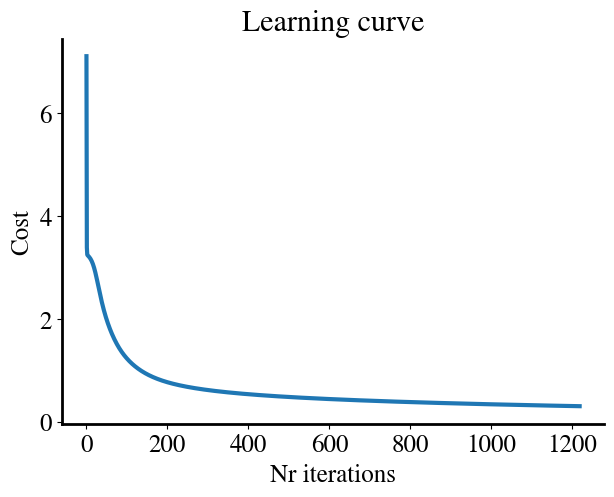
Even here, we can use the gradient descent method from the very first lecture on univariate linear regression to mimimize the ANN cost function:
Our own hard coded gradient descent method is nice because we can easily get whatever intermediate results we might be interested in, such as the errors at each iteration, which we can plot as the learning curve.
Code
if do_gradient_descent:
  plt.figure()
  plt.plot(range(i-1), errors[:i-1])
  plt.title('Learning curve')
  plt.xlabel('Nr iterations')
  plt.ylabel('Cost')
Accuracy on training data
Let’s look at the predictions for both the fast conjugate gradient and our slower gradient descent methods.
Code
# Evaluate trained model from conjugate gradient optimization (CG)pred_GC = nn_predict(all_theta_CG, input_layer_size, hidden_layer_size, num_labels, X)success_GC = np.mean(pred_GC == y) *100# Compute final costtotal_error = nn_cost(all_theta_CG, input_layer_size, hidden_layer_size, num_labels, X, y, lambda_r)print(f"Success rate of neural network with CG acceleration: {success_GC:.2f}%")print(f"Final cost: {total_error:.4f}")
Success rate of neural network with CG acceleration: 99.35%
Final cost: 0.1318
Code
if do_gradient_descent:# Predict using the trained theta vector pred_GD = nn_predict(theta_GD, input_layer_size, hidden_layer_size, num_labels, X) success_GD = np.mean(pred_GD == y) *100# Compute final cost GD_error = nn_cost(theta_GD, input_layer_size, hidden_layer_size, num_labels, X, y, lambda_r)print(f"Success rate of neural network with gradient descent: {success_GD:.2f}%")print(f"Final cost: {GD_error:.4f}")
Success rate of neural network with gradient descent: 96.45%
Final cost: 0.2998
As you can see, the ANN is extremely accurate on the training data. The reason that gradient descent seems slightly less accurate is because of the chosen tolerance. At the current tolerance, it will run the model in 1 minute but is a bit less accurate. If you make the tolerance 10 times smaller, it will take about half an hour to run but also achieve 100% accuracy on the training data.
Validation
Now test the neural network on the validation data set that was not yet seen by the algorithm:
Still very good performance on the validation data as well.
How to interpret an ANN? (optional)
While ANN are very good at modeling/predicting complex problems, it is notoriously hard to interpret how they actually do it when all these different layers compound and convolve ever more complexity.
If you try to google how to interpret these types of ANN for image recognition you will not find much. Below, I attempt to give you at least some more intuition of how the final tuned ANN makes predictions.
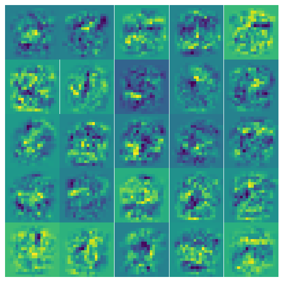
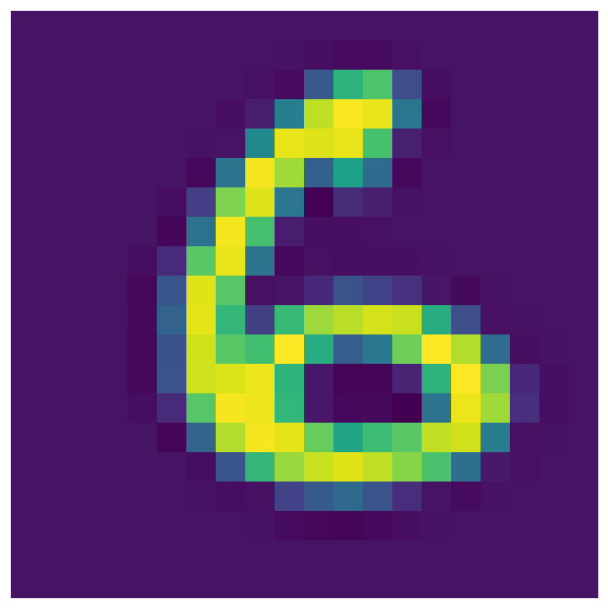
Let’s say we start with a single picture of a handwritten number and we want our ANN to predict what number it is. In the first step, each hidden node will get a different linear combination of the 400 pixes in the picture, in other words a different weighting of the importance of each pixel. We can visualize these weights \(\Theta^{[1]}\) directly as I do below. Each frame in this figure corresponds to one of the 25 nodes in the hidden layer, and the 20x20 pixels in each panel below correspond to the 20x20 weights that \(\Theta^{[1]}\) will give to the corresponding original 20x20 pixels in the picture.
In some sense, this step acts as a filter that will enhance some pixels and suppress others. Actually, it is applying 25 different filters; one will ‘brighten’ the pixels in the center-ish, another filter will enhance diagonal pixels etc. But in the end, it will add up all these weighted pixels and give one ‘score’ for each filter/hidden node.
In the hidden layer, each node ‘applies’ one of the 25 filters to this picture, if you will, and gives a ‘score’ ($ z = X $):
Code
X1 = np.append(1, xtry)z1 = X1.dot(Theta1_GC)print("The linear fit gives these hypotheses to the 25 hidden nodes:\n", np.reshape(np.round(z1,1),[5,5]))
The linear fit gives these hypotheses to the 25 hidden nodes:
 [[  2.7  -8.4  -2.2   7.5   3.3]
 [ -6.7  -4.9   8.9  -2.7  -4.8]
 [ -9.4  14.1   3.9   0.6   0. ]
 [ -6.5   1.7 -10.7  -1.4   6.4]
 [ -6.6 -13.4  11.1   3.6  -3.3]]
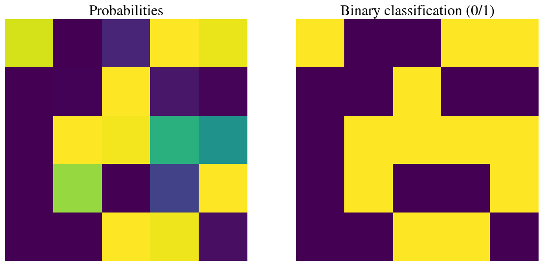
Next, the sigmoid function is applied to these scores. So what does that mean? The nodes that got a (large) negative score will get a weight of (near) zero and the nodes with a (large) positive score will get a weight of (near) 1.
Below, in the left panel, you can see these exact probabilities of each node (which, again, is like weighting different filters applied to this particular picture). The right panel shows what the corresponding true binary sigmoid predictions would be like, i.e. 1 for \(g(z)\ge 0.5\) and \(0\) for \(g(z)<0.5\).
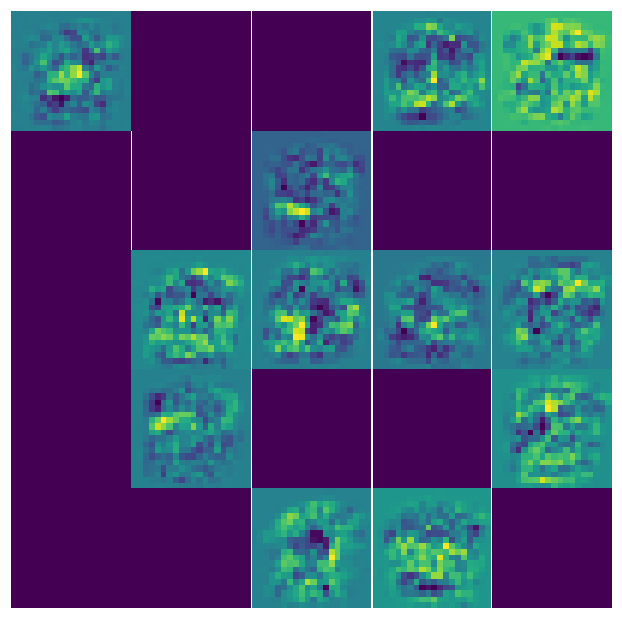
Finally, the last plot visualizes the \(\Theta^{[1]}\) weights/filters for each of the 25 nodes with \(g(z)\ge 0.5\).
Code
X2 = sigmoid(z1)print("The corresponding sigmoid gives probabilities to each of those combinations\n", np.reshape(np.round(X2,2),[5,5]))plota2 = np.reshape(X2,[5,5])fig, ax = plt.subplots(1,2, figsize=(14,7))# Probabilities:ax[0].pcolor(plota2)ax[0].invert_yaxis()ax[0].set_aspect('equal', 'box')ax[0].axis('off');ax[0].set_title('Probabilities');# Binary 1/0 classification:plota2 = np.where(plota2>=0.5, 1, plota2)plota2 = np.where(plota2<0.5, 0, plota2)ax[1].pcolor(plota2)ax[1].set_aspect('equal', 'box')ax[1].invert_yaxis()ax[1].set_title('Binary classification (0/1)');ax[1].axis('off');print("The corresponding sigmoid gives binary classification to each of those combinations\n", np.reshape(np.round(plota2,2),[5,5]))nrrows =5nrcols =5fig, axs = plt.subplots(nrrows, nrcols, figsize=(7, 7))for i inrange(nrrows):for j inrange(nrcols): idx = i * nrcols + jif idx >= hidden_layer_size: axs[i, j].axis('off')continue axs[i, j].pcolor(x_sq[:, :, idx][::-1, :] * plota2[i, j]) axs[i, j].set_aspect('equal', 'box') axs[i, j].axis('off')fig.subplots_adjust(wspace=0, hspace=0)plt.show()
The corresponding sigmoid gives probabilities to each of those combinations
 [[0.94 0.   0.1  1.   0.97]
 [0.   0.01 1.   0.06 0.01]
 [0.   1.   0.98 0.64 0.51]
 [0.   0.84 0.   0.2  1.  ]
 [0.   0.   1.   0.97 0.04]]
The corresponding sigmoid gives binary classification to each of those combinations
 [[1. 0. 0. 1. 1.]
 [0. 0. 1. 0. 0.]
 [0. 1. 1. 1. 1.]
 [0. 1. 0. 0. 1.]
 [0. 0. 1. 1. 0.]]
Note: a hidden node with output \(g(z)=0\) for the sigmoid function does not contribute any more at all to anything behind that hidden layer (if \(X^{[2]}=g(z)=0\) then \(X^{[2]}\cdot \Theta^{[2]}=0\) for any fitting parameter \(\Theta^{[2]}\) for that node).
For deep neural networks, in particular, where we can have multiple hidden layers, you may not want to completely kill off one of the neurons, i.e. the ones associated with nodes that have sigmoids of 0. This is where the alternative activation functions come in, such as the ‘leaky RELU’, which gives a probability close-to-but-not-exactly-zero to \(z<0\) and an ever larger probability \(g(z)\) for \(z>0\). That way, certain nodes/neurons can be given a small weight without completely eliminating them (their overal importance to the full network can still be determined to be relevant by the fitting parameters of subsequent layers). You may still want to use a sigmoid function for the output layer to only have probabilities between 0 and 1 for each classification (although a binary switch for \(g(z)\ge 0\) vs \(g(z)<0\) can also still be used for any activation function).
When moving from the hidden layer to the output layer/predictions, we again take linear combinations of the 25 numbers (\(g(z_2)\)) between 0 and 1 (as printed above) that were assigned to the hidden nodes. The results, \(\mathbf{z}^{[2]} = X^{[2]} \cdot \Theta^{[2]}\), are like a score for each possible prediction (that the picture is of a 0, 1, …, or 9):
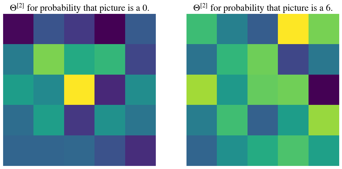
This mapping from the 25 hidden nodes to the 10 output nodes is done by the 26$$10 (induding the hidden bias) fitting parameters \(\Theta^{[2]}\). Visualizing all is maybe too much, but below I visualize the 25 fitting parameters (excluding the bias) in a 25$$25 color plot for 1) the output node that tests whether the picture is of a 0, and 2) the output node that tests whether the picture is the correct number (which is different each time you run this notebook).
The numerical values for all the fitting parameters \(\Theta^{[2]}\) are printed out as well. Note that negative values will reduce the importance of a given node to a given prediction (because of the sigmoid function that will be applied in the end) whereas positive numbers increase the importance of a given node for a given classification.
Code
Theta2_GCT = Theta2_GChidden_to_output_0 = Theta2_GCT[1:,0]hidden_to_output_correct = Theta2_GCT[1:,np.argmax(z3)]fig, ax = plt.subplots(1,2, figsize=(14,7))# Weights for output node picture is a 0:plota2 = np.reshape(hidden_to_output_0,[5,5])ax[0].pcolor(plota2)ax[0].invert_yaxis()ax[0].set_aspect('equal', 'box')ax[0].axis('off');ax[0].set_title(r'$\Theta^{[2]}$'+' for probability that picture is a 0.');# Weights for output node picture is a [correct number] (changes each time):plota2 = np.reshape(hidden_to_output_correct,[5,5])ax[1].pcolor(plota2)ax[1].set_aspect('equal', 'box')ax[1].invert_yaxis()ax[1].set_title(r'$\Theta^{[2]}$'+' for probability that picture is a '+str(np.argmax(z3))+'.');ax[1].axis('off');for i inrange(num_labels):if i == np.argmax(z3):print("Weights Theta2 from 25-node hidden layer to probability that picture is "+str(i)+': [correct number!]\n', np.reshape(np.round(Theta2_GCT[1:,i],0),[5,5]))else:print("Weights Theta2 from 25-node hidden layer to probability that picture is "+str(i)+':\n', np.reshape(np.round(Theta2_GCT[1:,i],0),[5,5]))
Weights Theta2 from 25-node hidden layer to probability that picture is 0:
 [[-3. -1. -2. -3. -1.]
 [ 0.  3.  2.  2. -1.]
 [ 1.  1.  4. -2.  1.]
 [-0.  1. -2.  1. -0.]
 [-1. -1. -0. -1. -2.]]
Weights Theta2 from 25-node hidden layer to probability that picture is 1:
 [[ 0.  2.  0.  2.  3.]
 [-3. -0. -2.  1.  1.]
 [ 1.  0.  1.  2.  1.]
 [ 2.  2. -2. -1.  0.]
 [ 1.  3. -4. -2.  2.]]
Weights Theta2 from 25-node hidden layer to probability that picture is 2:
 [[-3. -0.  2.  2. -2.]
 [-2. -3.  2.  3. -3.]
 [-3.  1.  1.  0.  1.]
 [-1. -3. -0. -3. -1.]
 [ 2. -2.  2.  3.  4.]]
Weights Theta2 from 25-node hidden layer to probability that picture is 3:
 [[ 0.  4. -1.  0. -2.]
 [ 2. -2. -2.  1.  3.]
 [-2.  2. -2. -3. -3.]
 [-0. -5. -2.  2. -0.]
 [ 0.  3.  1. -0. -3.]]
Weights Theta2 from 25-node hidden layer to probability that picture is 4:
 [[ 1.  1. -1. -4. -1.]
 [-2.  3.  0. -2. -0.]
 [ 0.  4. -1.  2.  0.]
 [ 3. -1.  0.  0. -4.]
 [ 3.  0. -2.  2. -1.]]
Weights Theta2 from 25-node hidden layer to probability that picture is 5:
 [[-1. -3.  3.  1.  4.]
 [ 2. -2. -3. -2. -4.]
 [ 3. -0. -4. -2.  3.]
 [-1.  2. -1.  1. -3.]
 [-2. -1. -2. -2.  2.]]
Weights Theta2 from 25-node hidden layer to probability that picture is 6: [correct number!]
 [[ 1. -1. -2.  3.  2.]
 [-1.  1.  2. -3. -1.]
 [ 2. -0.  2.  2. -4.]
 [-1.  1. -2. -0.  2.]
 [-2. -1.  0.  1. -0.]]
Weights Theta2 from 25-node hidden layer to probability that picture is 7:
 [[-2. -2.  2. -2.  1.]
 [ 3.  2.  1.  0.  1.]
 [-1. -3. -1.  3. -2.]
 [-1. -2.  4. -2. -0.]
 [-0.  2.  1. -3.  1.]]
Weights Theta2 from 25-node hidden layer to probability that picture is 8:
 [[ 4. -0. -3. -2. -3.]
 [-3. -2.  4. -1.  2.]
 [-3.  1. -2. -1.  2.]
 [-2.  3. -2. -3.  0.]
 [-0. -1.  1. -4. -1.]]
Weights Theta2 from 25-node hidden layer to probability that picture is 9:
 [[ 1. -0. -1. -1. -1.]
 [-1. -2. -1.  3. -1.]
 [ 0. -5. -1. -1.  1.]
 [ 1.  2.  2.  2.  3.]
 [-3. -3. -2.  3. -4.]]
In a sense, each of the figures above (or the numerical values printed) is again a mask or a filter applied to the result from the previous one in the hidden layer. The output from the hidden layer was visualized ealier has 25$$25 values of 1 or 0, i.e. yes or no. The 10 masks/filters above essentially sum up the yesses and nos with different weights corresponding to each outcome 0, 1, …, 9. Ideally, only one of those linear combinations is positive and all the others are negative. Here are those scores again:
Code
print("Scores z3 for output nodes 0, 1, ..., 9:\n", np.round(z3,0))
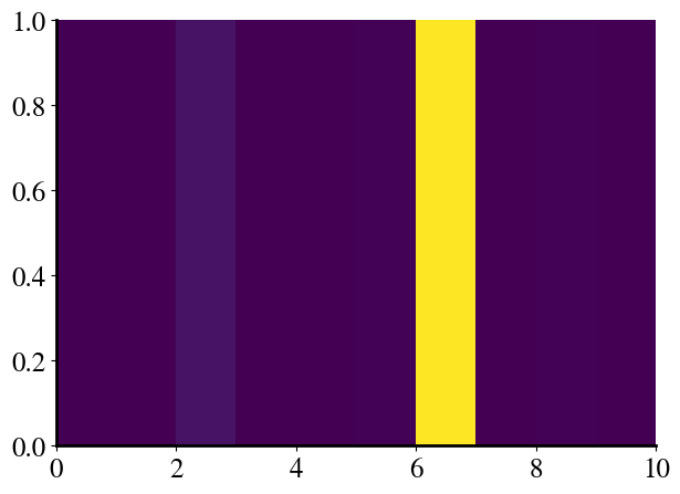
In that case, when we apply to final sigmoid function to the output layer, only one class will have a probability close to 1. The class with the highest probability (max\((g(z^{[3]}))\), or np.argmax(h3)) determines how the ANN classifies this example picture (note that I sneakily already used the correct number above by looking for the maximum value of \(\mathbf{z}^{[3]}\) itself, which will give a sigmoid value closest to 1):
Code
h3 = sigmoid(z3)correct_nr = np.argmax(h3)print("The probabilities that this picture is a 0, 1, ..., 9 are:\n", \ np.round(h3,3), '\n\nSo the most likely classification is:', correct_nr , \"\n\nOr graphically, these are the values of the 10 output nodes:\n")toplot = np.zeros([1,10])toplot[0,:] = h3plt.figure();plt.pcolor(toplot);
The probabilities that this picture is a 0, 1, ..., 9 are:
 [0.    0.002 0.048 0.    0.    0.005 0.994 0.    0.005 0.001]

So the most likely classification is: 6

Or graphically, these are the values of the 10 output nodes:
I realize that all this probably still does not make this ANN super easy to interpret…
Unfortunately, that is a well-acknowledged weakness of all types of neural networks, their lack of interpretability.