Which platform should I choose?

✏️ After this lecture, try the Practice exercise

Linear Regression, Cost Function, and (Accelerated) Gradient Descent

Note that you can collapse/expand individual sections. The ‘boring’ section below, for instance, has been collapsed to go straight to the more relevant materials.

Load various python libraries

First I load a bunch of external libraries. Only a small fraction of the libraries below are actually used in this notebook, but I just use the same ‘preamble’ in all my notebooks so I have access to all the libraries I frequently end up using. If you were to delete all of them, the following error messages in other cells will let you know which libraries to add back in.

from __future__ import division
import numpy as np
import matplotlib.pyplot as plt

# from matplotlib import animation
from IPython import display
import scipy.sparse as sp
import scipy.sparse.linalg
from scipy.linalg import solve_banded
from scipy import optimize

import time

%matplotlib inline
# %matplotlib notebook
from IPython.core.debugger import set_trace
plt.rcParams['figure.dpi'] = 100
plt.rcParams.update({'font.size': 18, 'font.family': 'STIXGeneral', 'mathtext.fontset': 'stix'})
# plt.rcParams['text.usetex'] = True
import pandas as pd


from IPython.display import clear_output
from time import sleep

small = 0.0000000001

Generate synthetic data for univariate linear regression

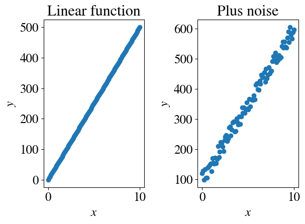
In this tutorial, we will work with the most trivial of data to develop a deep understanding of how various machine learning regression algorithms work. Specifically, we start with a target y (the dependent variable that we want to predict) on a single feature x (the independent variable). Moreover, we assume that the dependence is linear. Together, that defines a univariate linear regression problem.

Mathematically, we have \(y = \theta_0 + \theta_1 x\) and for noisy data \((x,y)\), the objective is to find the best fit for the intercept \(\theta_0\) and slope \(\theta_1\), such that the linear equation ‘matches’ (fits) the current data \((x,y)\) and of course predicts any future \(y\) given a condition \(x\). (You can think of some application in your Earth Sciences subfield as an example. For example, \(y\) could be the density of water as a function of concentration of dissolved salts \(x\)).

Implementationwise: the cell below generates some synthetic data to consider (in other words, data similar to something you might have measured in the field/lab). It also shows some of the functions that we will use a lot. Some of those are from numpy for Matlab-like calculations, and some from matplotlib for Matlab-like plotting.

First, we choose a number of measurement points. The default is a small number, such that everything runs very fast. Typical ML problems involve ‘big data’, though, and below we will mimic an algorithm specifically for massive data.

np.linspace(a,b,c) is the numpy version of linspace in Matlab. It simply creates a vector (technically, rank-1 array) with c equally spaced numbers between a and b.

Evertying starting with plt has to do with the plotting library. plt.subplot(a, b, c) means that we want an array of a rows and b collumns of (sub)plots, and currently we are plotting the c-ed plot in this table of (sub)plots (going first through row 1, then row 2 etc). For example, in the cell below: plt.subplot(1, 2, 2) refers to plotting the second plot (the last number) in a single row and 2 columns of plots.

Hopefully, the plt.scatter, plt.xlabel, plt.ylabel, plt.title commands are clear.

The numpy function np.random.uniform is used to add random ‘experimental’ errors to the data. There are two options to choose from: an absolute error (in the example above, say, \(\pm\) 3 kg/m\(^3\) error in density) or a relative error of, say, \(\pm 4\%\) which implies larger absolute errors at larger values of \(x\).

Feel free to try both options, and play with the magnitude of the errors.

Perhaps useful to point out: the # symbol ‘comments out’ lines in python, meaning they will be ignored. This allows one to add comments throughout one’s code, which is a very important coding best-practice. In these jupyter notebooks, the code and formatted text are separated more elegantly. Finally, the coding of the axes labels looks more complicated than it needs to be; this is to make publication-quality (latex-like) math symbols (e.g., italic). Simple labels are show below, commented out.

nr_measurements=100

abs_noise = True

x = np.linspace(0,10,nr_measurements)

############################################################
plt.subplot(1,2,1)
y = 50*x

plt.scatter(x,y)
plt.title('Linear function')
# Nicely formatted math symbols in axes lables:
plt.xlabel(r'$x$')
plt.ylabel(r'$y$')
# Simple labels:
# plt.xlabel("x")
# plt.ylabel("y")

############################################################
plt.subplot(1,2,2)
if abs_noise:
  y = 100 + y + np.random.uniform(-25,25,x.shape)
else:
  y = 100 + y * (1+ np.random.uniform(-0.1,0.1,x.shape))

plt.scatter(x,y)
plt.title('Plus noise')
plt.xlabel(r'$x$')
plt.ylabel(r'$y$')

plt.tight_layout()

If we assume that ‘true’ or physical/mathematical relationship between \(x\) and \(y\) is indeed linear, and more specifically given by our known definition $y = 100 + 50 x $ (see definition in code cell), then we can calculate the ‘experimental error’ of our syntetic data (with the added noise) with respect to that ‘correct’ model.

sq_measurement_error = mean_squared_error(100+50*x , y)/2
print("Measurement error is", sq_measurement_error)

Measurement error is 120.05123932176515

Exercise: modify the subplot lines in the cell two above to plot 2 rows of 3 figures (just copy-paste existing plots to fill in).

Linear fit with single loop for slope (brute force)

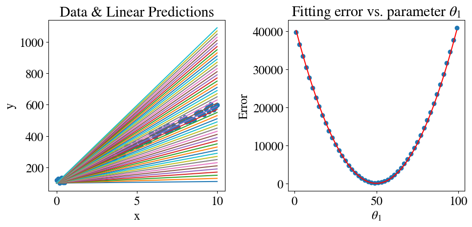
Below is an illustration of how one might naively implement the linear regression algorith. For the very simplest case, assume that we already know the intercept (\(\theta_0\)). This is often the case when we know the data should go through the origin \((0,0)\), for instance, but in this case we just set \(\theta_0 = 100\) from the definition above. All we will do is to try nrfits = 50 different values for \(\theta_1\) and see which provides the best fit.

There is a new numpy function introduced here that we will often use: np.zeros(nr_cols) generates a rank-1 array (a row vector) of size nr_cols with all its elements zero. The purpose is to ‘allocate’ enough memory for a variable before filling in all the non-zero values; plus, we cannot use index notation if a variable was not defined as a numpy array. The lab will go over other examples of vector- and matrix-type arrays of different dimensions.

Here, we define two rank-1/vector-type arrays: one will hold the 50 values of \(\theta_1\) that we try to fit and the other will store the fitting error of each of those values, such that we can visualize those.

We also see another one of the main programming concepts: the ‘loop’. You can see how this is usually done in python: for i in range(50): does the following. range is a python object that holds a list of integer values. If a starting number is not given, range(5) = 0, 1, 2,3, 4. In other words, by python convention, it starts at 0 and (to be consistent) does not include the last number. The specific loop in the cell below means that the body of the loop, which is everything that is indented after the colonm, will be executed 50 times. The for loop does not need an end statement as in other languages, because the end is automatically implied by the first line that is not indented.

The variable i is the iterator variable that is automatically incremented by one in each iteration of the loop. Sometimes that variable is used (for instance, to print how many times the loop body has been executed; you can uncomment the line below to test that), sometimes it is not. In the cell below, the iterator i = 0, 1, …, 49 is only used to construct the different values of \(\theta_1\) to try.

👉 Exercise: comment out that line (theta[i] = 1 + i*2) as well as the theta = np.zeros(nrfits) line, and instead use np.linspace to directly define a list of suitable \(\theta_1\) values to try.

Hint/reminder: you can always (temporarily) add a new code cell anywhere to try some things out before modifying more complicated cells. For instance, create a new cell and just see what np.linspace(10,1000,50) generates.

The cell below also shows how to modify fontsizes of plot labels (and similar for titles etc), and to format math symbols in the text.

Finally, it shows how by simply adding %%time to a cell, it will show you how much CPU (and wall) time it needs to execute, which is of course useful in comparing various algorithms.

%%time
plt.subplots(1,2,figsize=(10,5))
plt.subplot(1,2,1)

theta0 = 100 # assume a known/fixed intercept (also called bias)
nrfits = 50

errors = np.zeros(nrfits)
theta  = np.zeros(nrfits)

plt.scatter(x,y)

for i in range(nrfits):
    theta[i] = 1 + i*2
    y_pred = theta0 + theta[i]*x
    plt.plot(x,y_pred)
    errors[i] = mean_squared_error(y_pred , y)/2
    # print(i, "Trying theta1=", theta[i], "gives error", errors[i])

plt.title('Data & Linear Predictions')
plt.xlabel('x')
plt.ylabel('y')

plt.subplot(1,2,2)
plt.scatter(theta,errors) # errors are plotted as circle symbols

# We can also calculate the error in a different way:
# Mean squared sum of all x-es is constant:
mean_sq_x = x.dot(x)/(2*len(x))
# Error is square of difference between true and fitting theta (see also lecture notes)
# times the mean squared x (the noise does not even matter here):
error_th = mean_sq_x*(theta-50)**2

plt.plot(theta,error_th, color='r') # theoretical computed error is plotted as solid line

plt.title('Fitting error vs. slopes '+r'$\theta_1$')
plt.xlabel(r'$\theta_1 $')
plt.ylabel('Error')

plt.tight_layout()

# Save results for later
errors_sv = errors
theta_sv = theta

CPU times: user 152 ms, sys: 4.2 ms, total: 156 ms
Wall time: 154 ms

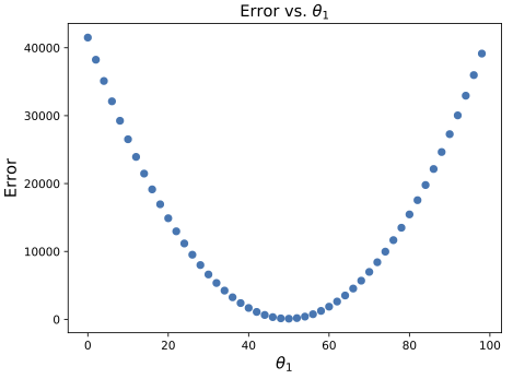
The figures are intented to show the clearest possible interpretation of how this “brute force” regression approach works: we try a number of parameters \(\theta_1\), each of which would ‘predict’ the linear \((x,y)\) dependence shown in the left plot with an associated error as shown in the right plot. Obviously, the errors are very high for very low \(\theta_1\) (as in far below the true slope), then the errors get smaller as we approach the correct slope, and then they increase again when we try slopes that are too high.

❓ What does the shape of the error plot look like? Any idea why?

The errors will be discussed in more detail below, but as a preview:

For this simple case, we can compute the errors directly. If we ignore the noise (which is less important than these very “wrong” guesses), the true

\(y_i = 100 + 50 x_i \quad \text{for } i=1,2,\ldots,m\)

and our predictions are

\((y_\mathrm{pred})_i = 100 + \theta_1 x_i\)

(because we already assume the correct intercept \(\theta_0 = 100\) in this first example).

The error can then be directly found as

\(\frac{1}{2m} \sum_{i=1}^m \big( (y_\mathrm{pred})_i - y_i \big)^2 = (\theta_1 - 50)^2 \; \frac{1}{2m} \sum_{i=1}^m x_i^2.\)

This is a simple quadratic function in \(\theta_1\) with the overall factor given by (half) the squared length of vector \(x\).

So how did we do? Search through all the errors we computed, find the iteration with the smallest error, and then find the value of \(\theta_1\) that corresponds to that minimum error.

min_ind = np.where(errors==np.min(errors)) # Note this very compact notation in python

besttheta = theta[min_ind[0]]

print("Minimum fitting/prediction error is:", round(np.min(errors),2), 'theta1 =', besttheta[0])

Minimum fitting/prediction error is: 124.51 theta1 = 49.0

We find that

1. The error is not that small for the best fit of \(\theta_1=49<50\),
2. It is clear that the algorithm is not that efficient: we used many iterations with guesses for \(\theta_1\) that were far from the correct one.

More specifically, the approach is naive in the sense that all of our guesses are equally spaced and don’t ‘zero in’ or ‘converge’ to the best fit in any kind of clever way. For similar reasons, this approach is sensitive to the upper and lower limits that we put on our guesses. If we knew that the correct slope was close to 50 (which we can see from just plotting the data), then we could use the same number of iterations but over a smaller range to get a more accurate solution (but the approach is still equally inefficient).

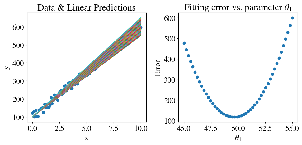
Let’s quickly try this below, which also shows the answer to the suggested exercise above: we define the \(\theta_1\) guesses as 50 equally spaced values between 45 and 55 using linspace.

plt.subplots(1,2,figsize=(10,5))
plt.subplot(1,2,1)

theta0 = 100
nrfits = 50

errors = np.zeros(nrfits)
theta = np.linspace(45,55,50)

for i in range(nrfits):
    y_pred = theta0 + theta[i]*x
    plt.plot(x,y_pred)
    errors[i] = mean_squared_error(y_pred , y)/2

plt.scatter(x,y)
plt.title('Data & Linear Predictions')
plt.xlabel('x')
plt.ylabel('y')

plt.subplot(1,2,2)
plt.scatter(theta,errors)

plt.title('Fitting error vs. parameter '+r'$\theta_1$')
plt.xlabel(r'$\theta_1 $')
plt.ylabel('Error')

plt.tight_layout()


min_ind = np.where(errors==np.min(errors))
besttheta = theta[min_ind[0]]

print("Minimum fitting/prediction error is:", round(np.min(errors),2), 'theta1 =', besttheta[0])

Minimum fitting/prediction error is: 117.86 theta1 = 49.69387755102041

If you compare the figures to the ones above, in the left of course you see that all the lines are closer to the data points and in the right you see that the errors are much smaller (especially on the ‘left’ and ‘right’), but we still missed the correct value of \(\theta_1=50\) simply because it was not in our vector of equally spaced test values.

Exercise: modify the cell above to try (perhaps even smaller number of) guesses that include \(\theta_1=50\).

Linear fit with double loop for slope and intercept (brute force)

To properly fit a linear model, we need to fit for both a slope and the intercept. The naive, or brute force, generalization of the previous section is to now use a double, or nested, loop. In the code below, we try 100 intercepts between 0 and 200, and for each of those guesses we try 100 slopes between 0 and 100. In total, that means \(100\times 100 = 10,000\) fitting trials, with again many of the combinations far away from the true answer.

Notice another trick that also introduces some useful python operations: the percentage sign is python for the ‘modulus’. To make the plotting below clearer, I only plot every 20eth iteration in j for \(\theta_0\) (meaning modulus(j,20)=0) and 20eth iteration in i. The notation for if statements is similar to for loops in the sense that the line ends with a colon, and whatever body is conditional on that if statement needs to be indented (the if statement is terminated by the first line that is not indented). A few more important details:

• you see that parantheses are not needed around the conditions of the if statement.
• the == statement does mean: is-exactly-equal-to, in contrast to the single = to assign some value (on the right) to a variable name (on the left). Example: if you assign a=1 and c=3 and b=c-2, then a==b will evaluate to True, because c-2 (with the value 3 assigned to c) will evaluate to 1, which was assigned to b. In other words, a and b are both just names for the number 1, so if we check if a and b refer to the same number, we use a==b.
• you see that you can simply write and or or to combine multiple conditional statements (as you may have practiced in the kaggle tutorial).

%%time
f, axs = plt.subplots(1,2,figsize=(12,5))
plt.subplot(1,2,1)

nrfits = 100

errors = np.zeros([nrfits+1,nrfits])
theta  = np.zeros(nrfits+1)
theta0 = np.zeros(nrfits)

tries = 0
for j in range(nrfits):
    theta0[j] = j * 200/nrfits
    for i in range(nrfits+1):
        theta[i] = i * 100/nrfits
        y_pred = theta0[j] + theta[i] * x
        if j % 20 == 0 and i % 20 == 0 :
            plt.plot(x,y_pred)
        errors[i,j] = mean_squared_error(y_pred , y)/2
        tries = tries+1

plt.scatter(x,y)
plt.title('Data & Linear Predictions')
plt.xlabel('x') # just basic arial labels this time, no fancy latex formatting
plt.ylabel('y')

min_ind = np.where(errors==np.min(errors))
besttheta0 = theta0[min_ind[0]]
besttheta1 = theta[min_ind[1]]

plt.subplot(1,2,2)
plt.scatter(x,y)
plt.plot(x,besttheta0+besttheta1*x,color='r')
plt.title('Best fit')
plt.xlabel('x')
plt.ylabel('y')

plt.show()

print("Minimum fitting/prediction error is:", round(np.min(errors),2), "after trying", tries, "combinations of fitting paramters ")
print("for theta0, theta1:", besttheta0[0], besttheta1[0])

errors_2D_sv = errors

Minimum fitting/prediction error is: 118.09 after trying 10100 combinations of fitting paramters 
for theta0, theta1: 98.0 52.0
CPU times: user 3.77 s, sys: 15.9 ms, total: 3.78 s
Wall time: 3.79 s

Again, we could change the lower and upper limits on both to use smaller intervals in our guesses to get a better fit.

The key point, though, is that we already used ~10,000 iterations for a completely trivial linear fit of 1 independent variable. In machine learning, we typically have dozens of independent variables to include in the fitting of \(y\).

As an aside, google colab adds a nice feature that after running a cell, if you hover your mouse over the ‘Play’ button, it shows you how long it took to run that cell. But also, explicit timing is added in these relevant cells for more precise timing (you see the difference can be quite significant).

I hope this long example drives home the message that we need more efficient algorithms to do even this simple type of fitting. In the next section, we therefore introduce the commonly used Gradient Descent Methods.

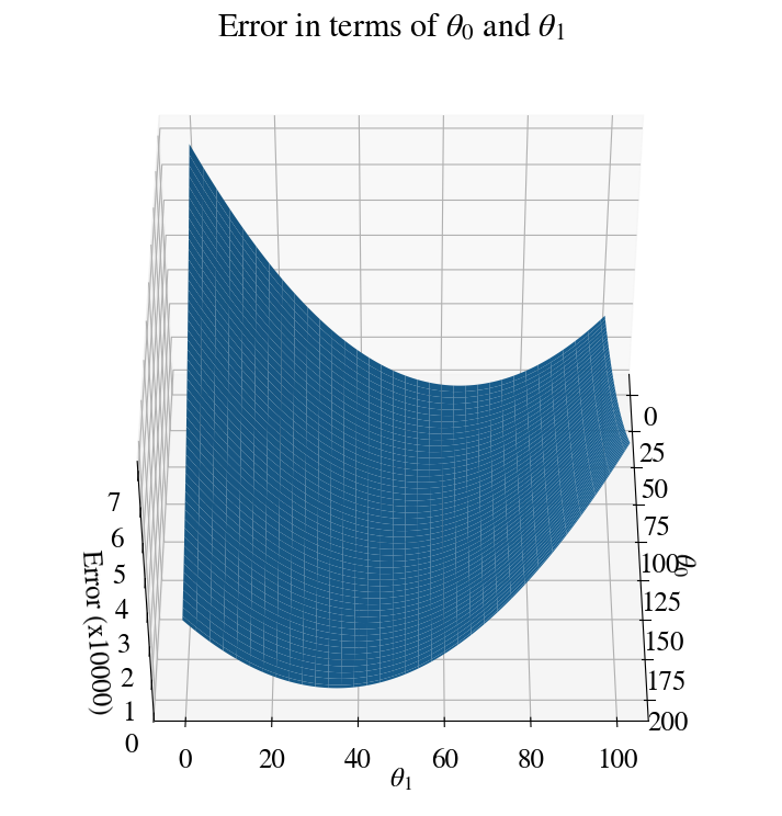
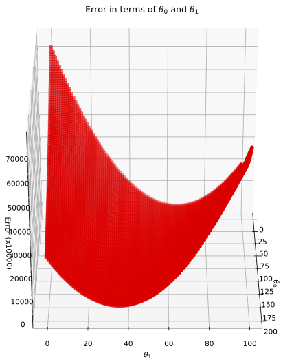
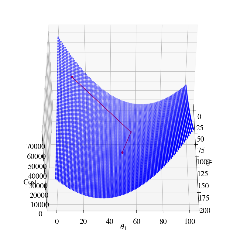
First, though, (because this will be important in the next sections) let’s have a look at the error for this example. The error is now a function of both \(\theta_0\) and \(\theta_1\) and therefore forms a surface in 3D space.

The cell shows how to create such a 3D surface plot and specify some view angle (the first number is kind of up/down, and the second one spinning around a vertical axis).

You also see how we need to make a mesh with np.meshgrid (just like the Matlab function with the same name) for every combination \((\theta_0, \theta_1)=\) error.

fig = plt.figure(figsize=(9,9))
ax = fig.add_subplot(111, projection='3d')
ax.view_init(45, 0)

T0, T1 = np.meshgrid(theta0, theta)

plt.title('Error in terms of '+r'$\theta_0$' + ' and ' +r'$\theta_1$')
ax.plot_surface(T0, T1, errors/10000)

ax.set_xlabel(r'$\theta_0$') # back to fancy axis labels
ax.set_ylabel(r'$\theta_1$')
ax.set_zlabel('Error (x10000)')

plt.show()

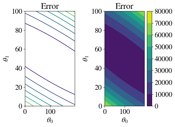
Another way to plot \(z(x,y)\) data is to use coloured or line contour plots.

plt.figure()

plt.subplot(1,2,1)
plt.contour(T0, T1, errors)
plt.xlabel(r'$\theta_0$')
plt.ylabel(r'$\theta_1$')
plt.title('Error')


plt.subplot(1,2,2)
plt.contourf(T0, T1, errors)
plt.colorbar()

plt.xlabel(r'$\theta_0$')
plt.ylabel(r'$\theta_1$')
plt.title('Error')

plt.tight_layout()

Hopefully it is clear that the fitting procedure corresponds to finding the minimum of this surface, i.e. the minimum fitting error. Notice, though, that the only reason I’m able to plot this surface at all is that I actually calculated the error for each of 10,000 \((\theta_0, \theta_1)\) pairs. Without doing so, the full form/shape of the error surface is not known and an efficient algorithm essentially tries to compute as little of it as possible. In other words, we want to find the minimal error with as few \((\theta_0, \theta_1)\) pair guesses as possible.

The following section discusses a first such method, which can also be applied to far more complex non-linear multivariate numerical regressions, as well as so-called logistical regressions that involve discrete categories (next weeks).

Gradient descent

The so-called gradient descent method is actually embarrasingly simple and obvious.

If you knew the slope of the error function, of course you would never pick a guess that is ‘up-hill’ along the error function, i.e. resulting in a larger error. If you started with some guess for \(\theta_1=25\) and knew the slope of the error at that point was negative, your next guess should not be \(\theta_1=20\) because that would definitely have a larger error. Similarly, for \(\theta_1=60\) the slope would be positive, so you wouldn’t need/want to try any larger values of \(\theta_1\). Instead, you always take a ‘little’ step ‘down-hill’ along the slope towards the minimum of the error function.

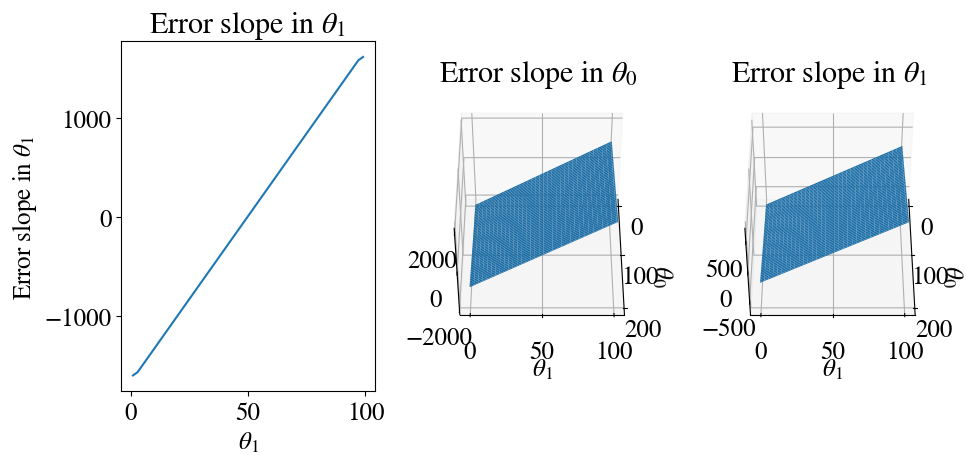
The slope of the error function is by definition its derivative. We can have a quick look at what these slopes look like by evaluating the numerical derivative of the errors using the np.gradient function. In our first example, the error was only a function of \(\theta_1\), whereas in the second example we considered both \(\theta_0\) and \(\theta_1\) so we need partial derivatives with respect to each.

# Gradient in theta1 when theta0 is kept constant:
error_slope = np.gradient(errors_sv, theta_sv)

# Gradient in both theta0 and theta1
[gx, gy] = np.gradient(errors_2D_sv)

# The rest is just plotting
fig = plt.figure(figsize=(10,5))
ax = fig.add_subplot(131)
ax.plot(theta_sv, error_slope)

plt.xlabel(r'$\theta_1$')
plt.ylabel('Error slope in '+r'$\theta_1$')
plt.title('Error slope in '+r'$\theta_1$')

# Gradient in theta0
ax = fig.add_subplot(132, projection='3d')
ax.view_init(45, 0)

ax.plot_surface(T0, T1, gx)
plt.xlabel(r'$\theta_0$')
plt.ylabel(r'$\theta_1$')
plt.title('Error slope in '+r'$\theta_0$')

# Gradient in theta1
ax = fig.add_subplot(133, projection='3d')
ax.view_init(45, 0)

ax.plot_surface(T0, T1, gy)
plt.xlabel(r'$\theta_0$')
plt.ylabel(r'$\theta_1$')
plt.title('Error slope in '+r'$\theta_1$')

plt.tight_layout()

As you can see, the slopes of the errors are linear functions in each direction. Importantly, for \(\theta\) smaller than the best fit, the slope is negative and for \(\theta\) larger than the best fit it is positive.

Hypothesis

In machine learning (ML) parlance, the first-order polynomial or linear model that we have used so far is the hypothesis \(h\) of our ML model. In other words, we want to predict \(\tilde{y} = h(x; \theta) = \theta_0 + \theta_1 x\). The notation \(h(x; \theta)\) means that our hypothesis \(h\) is a function of input values \(x\), and parameters (slope and intercept) \(\theta\).

Features

More machine learning lingo: our vector of independent variables \(x\) would be referred to as a single feature in this model. When we have more variables/features, we move into multi-variate linear (or later, non-linear) regressions.

Cost function

More machine learning (ML) lingo: instead of talking simply about fitting errors, those are referred to as the cost function or loss function, and instead of minimizing the error, we talk about minimizing the cost/loss.

At this point, we need to be a bit more specific about what error we have been using. As you can see from the intrinsic function name, we use the means_squared_error. If we consider \(m\) data points \(x_i=x_i, \ldots, x_m\) and we use some model to make predictions \(\tilde{y}_i\), while we also know the actual values \(y_i\), then the mean-squared-error (MSE) \(J\) is defined here as \(J = \frac{1}{2m} \sum_{i=1}^m (\tilde{y}_i - y_i)^2\).

This is also referred to as the L2 norm, while a similar definition in the absolute values is called the L1 norm or mean_absolute_error (which is also loaded): \(J = \frac{1}{2m} \sum_{i=1}^m |\tilde{y}_i - y_i|\).

The factor \(\frac{1}{2}\) is usually not there and included here specifically because if will cancel out a factor 2 when we take the gradient/derivative/slope of \(J\) later. We can add or remove any overall factor we want, because all we care about is finding where the minimum error \(J\) occurs, not what its actual value is (which is in arbitrary units here).

For our given hypothesis, the cost function can now be written explicitly as:

\(J = \frac{1}{2m} \sum_{i=1}^m (h(x_i,\theta) - y_i)^2 = \frac{1}{2m} \sum_{i=1}^m (\theta_0 + \theta_1 x_i - y_i)^2\)

This is a simple quadratic function in \(\theta_0\) and \(\theta_1\).

To clarify an important point that is easy to mix up at this point: * our hypothesis is a linear function in \(x\) which is defined by constant parameters \(\theta_0\) and \(\theta_1\); in other words, when our model is finished optimizing, we have found the best \(\theta_0\) and \(\theta_1\) and to predict any future values for a given condition \(x\), we just plug it into our hypothesis/model \(h(x,\theta)\) to predict the corresponding \(x\). * conversely, in the error function \(J(\theta)\) we consider a constant set of \((x,y)\) pairs and vary \(\theta\) to find its optimal value.

Cost gradient

With all the aforementioned definitions, we can define the cost gradients exactly. Let’s do this right away for both parameters (\(\theta_0\) and \(\theta_1\)):

• \(\frac{\partial J}{\partial \theta_0} = \frac{1}{m} \sum_{i=1}^m (\theta_0 + \theta_1 x_i - y_i)\).
• \(\frac{\partial J}{\partial \theta_1} = \frac{1}{m} \sum_{i=1}^m (\theta_0 + \theta_1 x_i - y_i) x_i\).

These partial derivatives are the slopes in the error landscape in the \(\theta_0\) (intercept) and \(\theta_1\) directions. If you think of a hilly topographical landscape, this would be equivalent to the slopes in the North-South direction (one dimension) and the East-West direction (a second dimensions).

Gradient Descent Method

We can now formally define the Gradient Descent Method (which we already described intuitively). Start with some/any initial guess for the pair (\(\theta_0\), \(\theta_1\)) and specify the one important “hyper-parameter” of this model: the learning rate \(\alpha\). Then, we improve our guess by take a small step ‘down-hill’ in each direction (a little bit down-hill in the \(\theta_0\) direction, and a little bit down-hill in the \(\theta_1\) direction, where ‘a little bit’ is defined by the learning rate \(\alpha\)). Specifically, we find new \(\theta_0^\mathrm{new}\), \(\theta_1^\mathrm{new}\) as:

• \(\theta_0^\mathrm{new} = \theta_0 - \alpha \frac{\partial J}{\partial \theta_0} =\theta_0 - \frac{\alpha}{m} \sum_{i=1}^m (\theta_0 + \theta_1 x_i - y_i)\),
• \(\theta_1^\mathrm{new} = \theta_1 - \alpha \frac{\partial J}{\partial \theta_1} =\theta_1 - \frac{\alpha}{m} \sum_{i=1}^m (\theta_0 + \theta_1 x_i - y_i) x_i\).

Then we set \(\theta_0^\mathrm{new}\) and \(\theta_1^\mathrm{new}\) as the new initial guess and repeat with another little step in the right direction. We can do this for a fixed number of steps (as implemented below), or should do so in a while loop until the results no longer improve (we have converged to the best solution for \(\theta_0\) and \(\theta_1\)).

It only takes a few lines to implement this entire algorithm (actually, we will make it even shorter and more efficient below).

%%time
nrsteps = 10000
thetas = np.zeros([nrsteps,2]) # test for yourself the shape of this array for a smaller value of nrsteps, like np.zeros([5,2])
errorsGD = np.zeros(nrsteps)

# Initial guess:
thetas[0,:] = [25,10]

# Step-size:
alphas = 0.01

for i in range(nrsteps-1):
    hypothesis = thetas[i,0] + thetas[i,1]*x
    errorsGD[i] = mean_squared_error(hypothesis,y) /2

    thetas[i+1,0] = thetas[i,0] - (10*alphas/len(y))  * sum(hypothesis - y) # I'm cheating here after some experimentation and to make nicer visualizations; I'm using a 10x higher learning rate in the theta0 direction, which one can do
    thetas[i+1,1] = thetas[i,1] - (alphas/len(y))  * sum((hypothesis - y)*x)

# Ssve result for comparison to other methods below:
theta_sv = thetas

CPU times: user 4.85 s, sys: 22.4 ms, total: 4.87 s
Wall time: 4.94 s

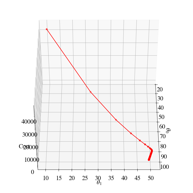
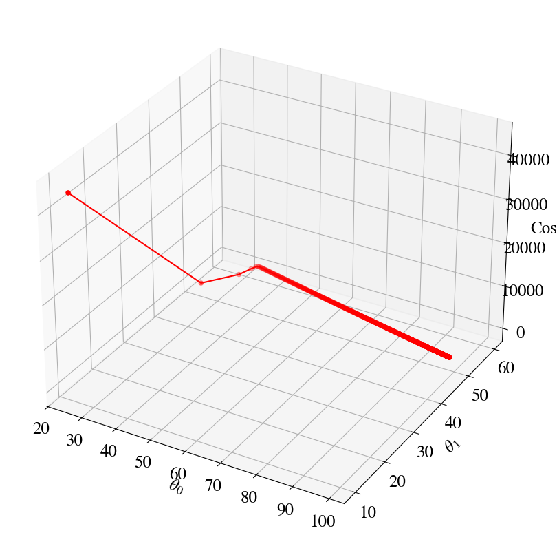
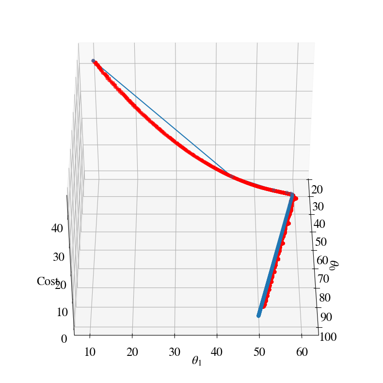
Let’s have a look at how it works in some plots. Here is the equivalent of the 2D surface of errors that we had before, but now you see how the errors ‘descent’ towards the minimum in a more ‘purposeful’ way:

fig = plt.figure(figsize=(10,10))
ax = fig.add_subplot(111, projection='3d')
ax.set_xlabel(r'$\theta_0$')
ax.set_ylabel(r'$\theta_1$')
ax.set_zlabel('Cost')

T00 = thetas[:,0]
T11 = thetas[:,1]

ax.scatter(T00, T11, errorsGD, c='r', marker='o')
ax.plot(T00, T11, errorsGD, color='r')

best0GD = round(T00[-1],2)
best1GD = round(T11[-1],2)

ax.view_init(45, 0)
print("Gradient descent error is", round(errorsGD[-2],2),\
      'with theta0, theta1',best0GD ,best1GD, 'after', nrsteps, 'steps.')
plt.show()

Gradient descent error is 117.42 with theta0, theta1 101.73 49.38 after 10000 steps.

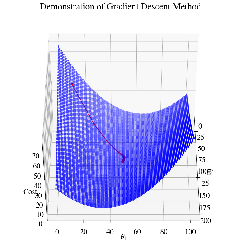
Let’s overlay the gradient descent result on top of the double/nested loop results (which computed the entire surface of errors). This illustrates how our Gradient Descent Method has us nicely ‘rolling down the error hills’ towards the minimum of the ‘error valley’.

fig = plt.figure(figsize=(10,10))
ax = fig.add_subplot(111, projection='3d')
ax.set_xlabel(r'$\theta_0$')
ax.set_ylabel(r'$\theta_1$')
ax.set_title('Demonstration of Gradient Descent Method')
ax.set_zlabel('Cost')

ax.scatter(T0, T1, errors/1000, c='b', marker='.')

ax.scatter(T00, T11, errorsGD/1000, c='r', marker='o')
ax.plot(T00, T11, errorsGD/1000, color='r')

ax.view_init(45, 0)
plt.show()

Just for python practice and/or to look at this from a different angle (pun intended) the same results are plotted below in 2D:

plt.figure()
plt.subplot(1,2,1)
plt.contour(T0, T1, errors)
plt.xlabel(r'$\theta_0$')
plt.ylabel(r'$\theta_1$')
plt.title('Cost')

plt.scatter(T00, T11, c='r', marker='o')
plt.subplot(1,2,2)
plt.contourf(T0, T1, errors)

plt.xlabel(r'$\theta_0$')
plt.ylabel(r'$\theta_1$')
plt.title('Cost')
plt.colorbar()
plt.scatter(T00, T11, c='r', marker='o')

plt.tight_layout()

Learning curve

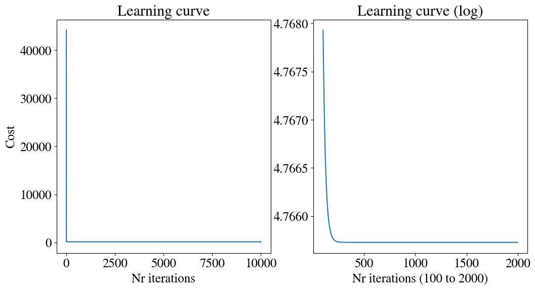
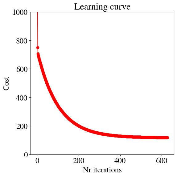
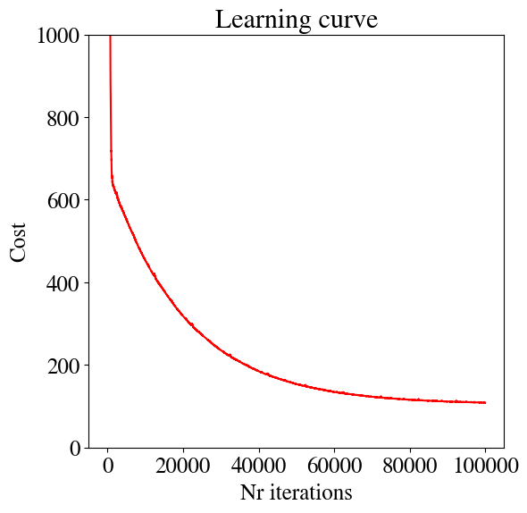
There are a number of ways to evaluate whether our machine learning algorithm is optimal and efficient, many of which will be discussed later. For now, let’s look at one simple one: the learning curve is simply a plot of the cost (fitting error) as a function of the number of iterations in our Gradient Descent. There are also other versions of learning curve. One is to plot the accuracy instead of the error/loss, with the accuracy increasing as the error/loss decreases. Another even more useful type of learning curve shows how the accuracy increases as we use more training data (discussed more later).

fig = plt.figure(figsize=(12,6))

plt.subplot(1,2,1)
plt.plot(range(nrsteps), errorsGD)
plt.xlabel('Nr iterations')
plt.ylabel('Cost')
plt.title('Learning curve')

plt.subplot(1,2,2)
plt.plot(range(100,2000), np.log(errorsGD[100:2000]))
plt.xlabel('Nr iterations (100 to 2000)')
# plt.ylabel('Log Cost')
plt.title('Learning curve (log)')

# plt.tight_layout()

Text(0.5, 1.0, 'Learning curve (log)')

You can see in the Learning Curve, and also by look more closely at the figures before it, that the error decreased very fast for the first few iterations and then very slowly for thousands of iterations in the end. This is partly due (as you can see from the figures) to the fact that the slopes in \(\theta_0\) and \(\theta_1\) have very different magnitudes. That is something that can be elleviated with ‘feature scaling’ (which will be discussed in another turorial). The other parameter that controls the efficiency is (obviously?) the learning rate \(\alpha\). For a larger learning rate, the algorithm will take bigger steps and this theoretically get to the minimum faster. However, you can image that if we take the steps to large, we can overshoot the minimum and end up on the up-slope on the other side of the valley. You can play around with \(\alpha\) to try an get the best efficiency, but intuitively, and from the figures, it is perhaps already clear that it would be useful if \(\alpha\) was chosen automatically based on the shape of the error function, and furthermore adaptive so it could take big steps where appropriate, but then ‘slow down’ to smaller steps when necessary. That is the conceptual idea behind accelerated optimization methods discussed later.

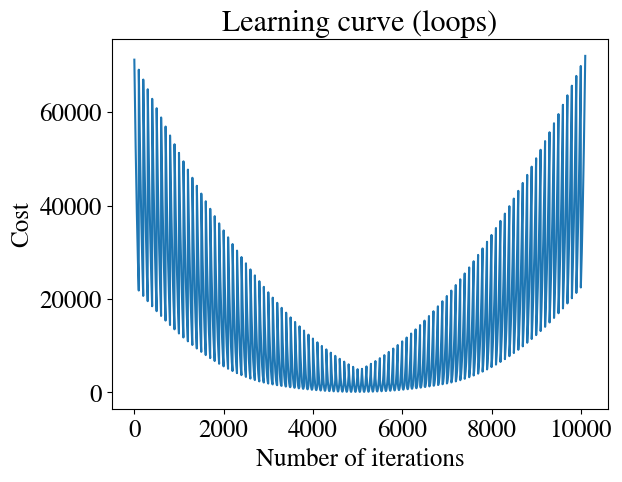
For comparison, let’s also take a look at the learning curve of the brute force double-loop fitting approach below. Clearly, there is no ‘learning’ involved here, as there is no convergence to a best solution. In a sense, this is the difference between some generic regression algorithm versus a “machine learning” algorith. The plot looks odd because for every guess of \(\theta_0\), we loop through our full range of \(\theta_1\) guesses, with the best guess happening somewhere in the middle of that range. For example, for the first 100 (and again the last 100) iterations, we use a very bad guess for \(\theta_0\), but the error first decreases and then increases again as we loop through guesses for \(\theta_1\). Then, we try an slightly better guess for \(\theta_0\) and again loop through \(\theta_1\), so all the errors are sill large, but a bit smaller than for the previous \(\theta_0\). The best \(\theta_0\) also happened to be in the middle of the range of guesses, so after around 5000 iterations we have the best guess for both \(\theta_0\) and \(\theta_1\). But without using some convergence criterion, we then still keep ploughing through the full range of bad guesses that we specified, with ever increasing errors.

loopsteps = np.size(errors)
error_prog = np.reshape(errors,loopsteps)
plt.plot(range(loopsteps), error_prog)
plt.xlabel('Number of iterations')
plt.ylabel('Cost')
plt.title('Learning curve (loops)')

Text(0.5, 1.0, 'Learning curve (loops)')

In the following, first we look at a few technical aspects that will be important when we generalize these methods to more complex problems.

Also, we will introduce a less sophisticated method, but one that is more efficient for extremely large datasets.

One last important comment on the learning rate: not all algorithms converge all the time. In other words, for some algorithms the solution may improve for a few steps, get worse for some steps, and then improve again (or in some cases, diverge, and get worse and worse). It can be shown, though, that because of certain properties of the cost funtion (namely that it is concave), the gradient descent method does move closer to the minimum cost (best fit) in every iteration. If we plot the learning curve and it goes up anywhere, that shows an error in implementation. Plotting the learning curve is therefore also a good test of coding (obviously, if the error always decreases in every iteration, we’re happy).

Vectorization

Matlab and python are both interpreter languages. That means that the code you write is translated into machine-readable code only when you run it. Compiler languages, like fortran, c, c++, etc., as the name suggests, need to be compiled into an executable (like a Windows ‘.exe’ file) before you can use/run your code. Intepreter languages are nice, because you execute a line of code as soon as you write it, but have some severe limitations in terms of efficiency that you always need to be cognizant of. There is a reason that compiler languages are the standard for ‘serious stuff’. Put simply, when you compile a fortran or c code, the compiler can spend some serious time figuring out how to turn your human-readable code into the most efficient machine-readable code. Hardware manufacturers, in particular, compete in making their compilers extremely efficient and squeeze every bit of power out of their CPUs (and GPUs). That involves taking into account all kinds of specific hardware specs that you would preferably never have to think about. As an important example: Moore’s law of computer speeds getting X times faster every so many years does not directly apply anymore in the old sense. Clock-speeds (the GHz advertised of your processor) have hardly increase for about a decade, and instead all speed increases come from having multiple CPUs and running software/codes in parallel, which is more or less synonymous with using multiple threads (hyperthreading). This is important in this context because compiler languages offer a wide range of sophisticated automatic parallelizations.

In contrast, an interpreter language like python has to translate each line of code you write into machine language while it runs (/executes) your code. The most important detrimental example of this is a loop. If you run a loop over 10,000 iterations, each iteration requires the same line of code you wrote to be translated into machine code. There are other operators, such as, say, the sum of the element-wise product of two vectors, that effectively also involve a loop over all the vector’s elements. Those operations are very slow in an interpreter language (python) versus a compiler language (fortran).

The solution, which can almost entirely overcome this issue, is to take clever use of linear algebra whenever possible. The reason is that Matlab and python have back-ends for many operations that are written in maximally optimized c-code. Example: a loop is hard to optimize because python does not know what the loop does; but if you want to computer the ‘sum of the element-wise product of two vectors’, this is the same as the mathematical/linear algebra dot-product of two vectors, and python (and Matlab) have highly optimized parallel code to do this. The same holds for anything that can be written as a vector-vector, vector-matrix, matrix-matrix (or higher dimensional arrays) multiplications, divisions, etc. To repeat: this is what is referred to as vectorizing your code, which leads to higher efficiency and often automatic paralellization (nowadays this is true even in compiler languages too).

As an example, we make just a tiny modification to the Gradient Descent code. We expand our feature array \(x\) by a feature that is always one (i.e., we just add a column of ones). If we had \(m\) (experimental) data points, \(x\) would now be a \(m\)-rows by \(2\) colums array. That means that we can directly multiply this array with the parameter vector \(\theta = [\theta_0, \theta_1]\) to get our hypothesis. Using bold for vectors/matrices/arrays: \(\mathbf{y} = h(\mathbf{x} , \mathbf{\theta})= \mathbf{x} \cdot \mathbf{\theta}\), where the dot is shown explicitly (not necessary) to denote vector-matrix multiplication.

Similarly, in matrix notation the cost gradient (denoted by \(\nabla = \left(\frac{\partial}{\partial \theta_0}, \frac{\partial}{\partial \theta_1}\right)\)) can be written in one line, one operation, as \(\nabla J = (h(\mathbf{x} , \mathbf{\theta}) - \mathbf{y}) \cdot \mathbf{x}\).

All this is done in the slightly revised code below. If you do the trick of hovering over the ‘Play’ icons, you’ll see that this code is about 17% faster than the non-vectorized code above and that’s probably without parallelization. The difference may not seem that significant but it also makes the code more ‘elegant’ and it will make the generalization to multi-variate regression more obvious/elegant as well.

%%time
nrsteps = 10000
m = len(y)
thetas = np.zeros([nrsteps,2])
errorsGD = np.zeros(nrsteps)

alpha_m = alphas/m

x_aug = np.zeros([m,2])
x_aug[:,0] = 1
x_aug[:,1] = x

# Initial guess:
thetas[0,:] = [25,10]

for i in range(nrsteps-1):
    hypothesis = x_aug.dot(thetas[i,:])
    errorsGD[i] = mean_squared_error(hypothesis,y) /2

    thetas[i+1,:] = thetas[i,:] -  alpha_m * (hypothesis - y).dot(x_aug)

print("Checking:")
print("Final theta0 and theta1 from nested loops were", besttheta0[0], besttheta1[0], \
      ', the results from the previous gradient descent were', best0GD, best1GD)
print('The results from the optimized gradient descent should be the same (but faster) at',  round(thetas[-1,0],2),round(thetas[-1,1],2))

Checking:
Final theta0 and theta1 from nested loops were 98.0 52.0 , the results from the previous gradient descent were 101.73 49.38
The results from the optimized gradient descent should be the same (but faster) at 101.73 49.38
CPU times: user 3.63 s, sys: 9.96 ms, total: 3.64 s
Wall time: 3.64 s

The vectorized formulation may also be safer to implement gradient descent. A common coding error is to implement the algorithm (see above) as:

• \(\theta_0 = \theta_0 + \alpha \frac{\partial J}{\partial \theta_0} =\theta_0 + \frac{\alpha}{m} \sum_{i=1}^m (\theta_0 + \theta_1 x - y)\),
• \(\theta_1 = \theta_1 + \alpha \frac{\partial J}{\partial \theta_1} =\theta_1 + \frac{\alpha}{m} \sum_{i=1}^m (\theta_0 + \theta_1 x - y) x\).

Can you even spot the difference?

In this implementation, \(\theta_0\) and \(\theta_1\) are updated ‘in place’ if you will; in other words we don’t save all the intermediate values but only the current ones, which are always the more accurate. The error in implementing it this way is that \(\theta_0\) is updated before \(\theta_1\) is. The new \(\theta_0\) would be used (inside the hypothesis) in the update of \(\theta_1\) which is inconsistent with how the gradients are defined, and may not always converge properly.

While-loop implementation

As mentioned before, using a for loop does not really make sense. On the one hand we don’t really know how many iterations we need to get an accurate enough fit; on the other hand, if we pick a very large number, we may already reach the most accurate fit early on and do many more iterations for no good reason. In the code below, we therefore use a while loop. We select our own tolerance parameters (as small number) and continue improving our fit until the cost function (error) improves less than that tolerance in a given iteration. While we’re at it, let’s also see if we can make the learning rate 2 times larger (\(\alpha=0.02\)).

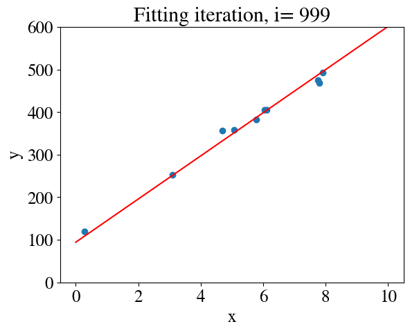
Before running the improve Gradient Descent method, let me define a function to plot the results, to keep the gradient descent code itself cleaner.

def my_plot(x_true,y_true,x_pred,y_pred,i,converged):
      plt.scatter(x_true,y_true)
      plt.plot(x_pred,y_pred,'r-')
      plt.ylim(0,600)
      plt.title('Fitting iteration, i= ' + str(i))
      plt.xlabel('x')
      plt.ylabel('y')
      plt.show()
      sleep(0.01)
      if(not converged):
        clear_output(wait=True)

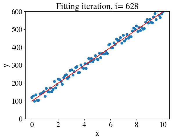
# %%time
nrsteps = 10000
m = len(y)
thetas = np.zeros([nrsteps,2])
errorsGD = np.zeros(nrsteps)

alpha = 0.02      # learning rate
alpha_m = alpha/m # overall factor is learning rate divided by nr of samples

x_aug = np.zeros([m,2])
x_aug[:,0] = 1  # bias feature for intercept
x_aug[:,1] = x

# Initial guess:
thetas[0,:] = [25,10]

i=0
converged = False
tolerance = 1e-4
plt.figure()
while not converged:
    hypothesis = x_aug.dot(thetas[i,:]) # model fit

    errorsGD[i] = mean_squared_error(hypothesis,y) /2

    thetas[i+1,:] = thetas[i,:] -  alpha_m * (hypothesis - y).dot(x_aug) # the last term is learning rate times error gradient
    if np.abs(1-errorsGD[i]/errorsGD[i-1]) < tolerance: # this just checks if we have converged to the most accurate fit
      converged = True

    # Plot results:
    if i<25 or i % 50 == 0 or converged:
        my_plot(x,y,x,hypothesis,i,converged)
    i+=1

print("Checking:")
print("Converged in", i, "iterations with thetas: ", thetas[i,:], "and error ", errorsGD[i-1])

print("Final theta0 and theta1 from nested loops were", besttheta0[0], besttheta1[0], \
      ', the results from the previous gradient descent were', best0GD, best1GD)
print('The results from the optimized gradient descent should be the same (but faster) at',  round(thetas[i-1,0],2),round(thetas[i-1,1],2))

Checking:
Converged in 629 iterations with thetas:  [98.69952368 49.83041683] and error  118.59061044832613
Final theta0 and theta1 from nested loops were 98.0 52.0 , the results from the previous gradient descent were 101.73 49.38
The results from the optimized gradient descent should be the same (but faster) at 98.68 49.83

Running this version, you see that out of the 10,000 iterations used above, we only need 1092 or less (depending on what we choose for learning rate). The code is now about/at least an order of magnitude faster than the one we started with.

Let’s see what the error landscape looks like:

thetas_batch = thetas[:i,:]
error_batch = errorsGD[:i]

fig = plt.figure(figsize=(10,10))
ax = fig.add_subplot(111, projection='3d')
ax.set_xlabel(r'$\theta_0$')
ax.set_ylabel(r'$\theta_1$')
ax.set_zlabel('Cost')

TT0 = thetas_batch[:,0]
TT1 = thetas_batch[:,1]

ax.scatter(TT0, TT1, error_batch, c='r', marker='o')
ax.plot(TT0, TT1, error_batch, color='r');

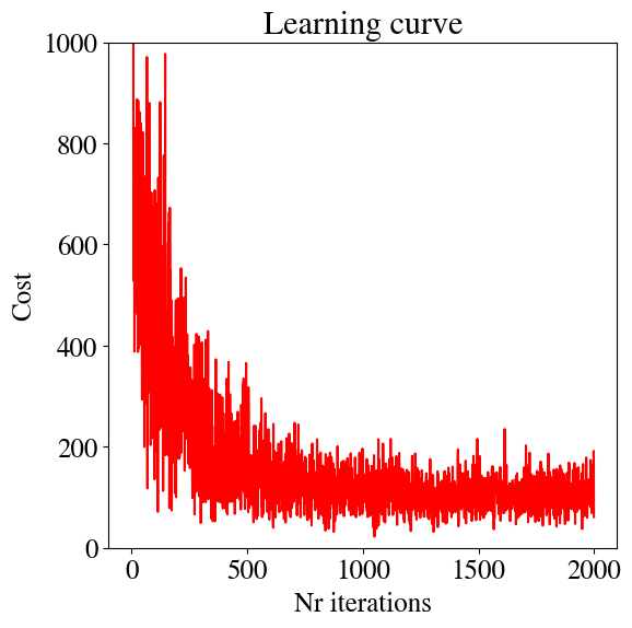
We can also look at the learning curve again. The first few errors are extremely large and result in a \(y\)-axis that obscures the smaller improvements at later times. For this reason, I set the vertical axis to a maximum range of MSE\(_\mathrm{max}\) = 1000

fig = plt.figure(figsize=(6,6))

plt.plot(range(i), errorsGD[:i],'r-o')
plt.xlabel('Nr iterations')
plt.ylabel('Cost')
plt.title('Learning curve')
plt.ylim(0,1000)

The learning curve shows how we gradually approach the minimum error and stop as soon as the errors plateau and don’t improve any further.

Advanced / Accelerated / Higher-Order Regression Methods (e.g., Newton)

Note: the technical details in this section may be a bit overwhelming if you haven’t taken linear algebra before. I provide it for those students who may be interested in fully understanding these fastest algorithms, but others will be fine without full understanding these details. The short version/summary is that by computing not only the first but also the second derivative of the error/cost/loss function, we can autimatically find the optimal learning rate, which automatically adjusts as we get closer to the smallest error / highest accuracy.

While the Gradient Descent Method is easy to implement and robust, it has two (related) weaknesses:

• The learning rate, \(\alpha\), is an ad-hoc number to define the step-size; choose it too big and it may overshoot the minimum, choose it too small and it will take many many steps before finding the best fit. Often, one has to just try several choices, re-run the entire regression, and find the most efficient rate.
• The learning rate is fixed, which is not effient. It often makes sense, for instance, to take a few big steps initially when fitting errors are large, but then take smaller and smaller steps as we approach the best fit. For instance, we could implement a linear reduction as alpha = alpha * (1 - i/nrsteps), but this is still not optimized for what the cost function for a specific problem looks like.

The answer to this question of how to optimize the learning rate is the (reciprocal of the) second derivative of the cost function. While the first derivatve gives the slope of the cost function (defing uphill and downhill), the second derivative provides the curvature of the cost function, which is an excellent indicator of how large of a step we can take.

To those of you familiar with the Newton method to find the roots (zeroes) of an equation, this is the same method but applied to a slightly different problem. Often Newton’s method is used to find the solution \(f(x) = 0\) for \(x\). Starting with some initial guess \(x^1\) and knowing the slope/derivative $ f^(x) = $, Newton’s method finds a better solution \(x^2 = x^1 - f(x^1) / f^\prime (x^1)\) (note that the superscripts are not powers, but an iterator of how one would do this in a loop). Python code would be:

while increment > tolerance:
  increment = func(x) / func_deriv(x)
  x = x - increment

which converges quadratically to the solution where \(f(x)=0\) (for every step, the error reduces by the square of the step-size).

In our numerical regressions, the problem is slightly different. We are typically not going to find a solution where the fitting error is zero. Rather, we try to find the mimimum of the error function. The minimum (or maximum) of a function implies a zero derivative. So, we’re not trying to find where a function is zero, but where that function’s derivative is zero. Still, if we define a function \(f(\theta) = \frac{\partial J(\theta)}{\partial \theta}\), with derivative \(f^\prime(\theta) = \frac{\partial^2 J(\theta)}{\partial \theta^2}\), the algorithm is exactly like the above.

In the above, we have written \(f\) and \(J\) as functions of only one variable. Even the univariate linear regression allready has 2 parameters, though: \(\theta_0\) and \(\theta_1\). When we consider multivariate linear regression with \(n\) features (including the \(x=1\) auxiliary feature), and thus \(\theta_0, \theta_1, \ldots, \theta_n\), we need a vector of first derivatives \(\nabla J = \left( \frac{\partial J}{\partial \theta_0} , \frac{\partial J}{\partial \theta_1} ,\ldots, \frac{\partial J}{\partial \theta_n} \right)\) and a \(n\times n\) matrix of second derivatives with components:

$ J = $ for all \(i=1,\ldots, n\), \(j=1,\ldots, n\). This matrix is called the Hessian.

The Newton accelerated linear regression algorithm is just the Gradient Descent method with the learning rate \(\alpha\) provided automatically by the inverse of the Hessian matrix. In vector/matrix notation we (schematically/pseudo-code) implement:

while increment > tolerance:
    improvement_step = inverse(Hessian) . gradient / m
    theta_new = theta - improvement_step
    increment = magnitude(improvement_step)

The Newton algorithm is very powerful (fast), but its implementation can be more daunting because of the need to evaluate all the second order partial derivatives in the Hessian. Moreover, if you remember your linear algebra, not every matrix has an inverse! In fact, even for our simplest linear problem, the Hessian of our cost function is \([[1, x], [x, x^2]]\), which doesn’t have an inverse. It is singular, because the second row is just \(x\) times the first row.

Fortunately, both the challenges of coding up the Hessian and issues with the inverse of the Hessian are handled automatically in libraries available in python (e.g., by using approximated Hessians that can be inverted and sometimes evaluating the Hessian numerically rather than exactly).

python has a very powerful library optimize, which includes a minimization procedure (optimize.minimize) that has multiple fast schemes to choose from. Below we use a (truncated) Newton method. As input, it only needs the cost function and its gradient, but we don’t have to code up the Hessian. The cost and its gradient need to be provided as function handles, so let’s define those functions first:

def cost(theta, x, y):
    hypothesis = theta[0] + theta[1]*x
    cost = sum((hypothesis - y)**2)/(2*len(y))
    return cost

def gradient(theta, x, y):
    hypothesis = theta[0] + theta[1]*x
    grad1 = sum((hypothesis - y))  /(len(y))
    grad2 = sum((hypothesis - y)*x)/(len(y))
    grad = [grad1, grad2]
    return grad

The optimized function does not automatically provide the intermediate results, which a user generally does not care about. To investigate and illustrate how the Newton method converges, though, we can use a so-called ‘call back’ function. The mimimization routine will call this function every iteration, so we can add some print statements to observe the results.

Note a new python feature here: the function needs some global variables. Using global variables inside a function, instead of explicitly passing those as inputs is generally a faux pas in coding and not advised. In this case, it is necessary though because of how the callback function is handled in python’s optimize function (which does not allow us to have any number of input variables for the call back function).

def callbackF(theta):
    global Nfeval, x, y,saveresults
    error = sum((theta[0] + theta[1]*x - y)**2)/(2*len(y))
    print('iter ={0:4d}   theta0 ={1: 3.6f}   theta1 ={2: 3.6f}   error ={3: 3.6f}'.format(Nfeval, theta[0], theta[1],error))
    Nfeval += 1

Doing the regression is now as easy as just calling the optimize function, with some initial guess of course:

%%time
theta0 = [25,11]
Nfeval = 1

result = optimize.minimize(cost, theta0, args=(x,y), method='TNC', jac=gradient, \
                           options={'disp': True}, callback=callbackF,tol=0.0001)


if result.success:
    besttheta = result.x
    nriterations = result.nit
    print("Converged after", result.nit, "iterations to best theta fits:", besttheta)
else:
    print("Accelerated method did not work, maybe try gradient descent.")

y_pred_NM = besttheta[0] + besttheta[1]*x
error_NM = mean_squared_error(y_pred_NM,y)/2
print("Error of accelerated method is:", round(error_NM,2))

iter =   1   theta0 = 58.974029   theta1 = 55.975769   error = 350.138737
iter =   2   theta0 = 101.304073   theta1 = 49.164278   error = 118.697072
iter =   3   theta0 = 101.726195   theta1 = 49.375326   error = 117.416437
Converged after 3 iterations to best theta fits: [101.7261949   49.37532599]
Error of accelerated method is: 117.42
CPU times: user 3.25 ms, sys: 0 ns, total: 3.25 ms
Wall time: 3.23 ms

As you can see, the algorithm is pretty amazing. It converges in only two or three steps! Remember, we started with an algorithm that used 10,000 steps and still finished with a larger error than the above.

Let’s visualize this:

fig = plt.figure(figsize=(10,10))
ax = fig.add_subplot(111, projection='3d')
ax.set_xlabel(r'$\theta_0$')
ax.set_ylabel(r'$\theta_1$')
ax.set_zlabel('Cost')

T00 = [25,59.186998,102.812541,103.264482]
T11 = [10,56.209235,49.182097,49.403970]
errorsGD = [cost(theta0,x,y), 358.051538,112.103335,110.675238]

ax.scatter(T00, T11, errorsGD, c='r', marker='o')
ax.plot(T00, T11, errorsGD, color='r')

ax.scatter(T0, T1, errors, c='b', marker='.')
ax.view_init(45, 0)

You can see that the Newton algorithm ‘knew’ exactly how large to take one maximum step to descend the steep hill in the \(\theta_1\) direction, followed by one optimal step mostly down the \(\theta_0\) slope.

Further reading: ( https://scipy-lectures.org/advanced/mathematical_optimization/index.html )

Stochastic Gradient Descent

There is one more regression algorithm I want to introduce you to before switching to nonlinear and multivariate regressions, which is called stochastic gradient descent. Let’s still consider the simplest case of a linear model for one feature x, such that we optimize only two parameters \(\theta_0\) and \(\theta_1\).

For the appropriate context, remember how regular gradient descent (and even the naive nested loops approach) work. We start with some initial guess for \(\theta_0\) and \(\theta_1\) and then we compare the linear prediction \(\tilde{y}_i\) to the measured \(y_i\) in terms of their squared distance/error. Notably, we do this for every measurement point \(x_i = x_1, x_2, \ldots, x_m\) and take the sum of all those errors to obtain the total fitting error associated with that choice of \(\theta_0\) and \(\theta_1\). Then we do the same thing again and again, iterating sometimes hundreds of steps to find the optimal \(\theta_0\) and \(\theta_1\). Similarly, in updating \(\theta\), we consider the gradient of the cost function at every point \(x_i\).

When we have massive amounts of data, say 100 million measurements (\(m=10^6\)), evaluating the cost function and its gradient for all \(m\) points in each iteration can become not only computationally expensive, but may even run out of memory.

Stochastic gradient descent is a method specifically developed for such massive datasets. At every iteration (meaning, every attempt to find better values for \(\theta\)), stochastic gradient descent only looks at one of the points and it makes an \(\alpha\)-sized step down-gradient that only considers improving the fit to thay specific point. In the next iteration, it does the same thing, but for another point, and then another point. In doing so, it slowly meanders around, more or less in a random-walk, but still ends up circling the minimum of the cost function and associated best fit (I won’t distract you with the mathematical argument/proof that this approach still converges to the optimal solution). This approach is much less accurate per-step and may need many more steps than regular gradient descent (which is also called batch gradient descent, because it fits the entire ‘batch’ of all \(m\) data-points at once). However, each individual step takes much less time and memory, which wins out for very large \(m\).

As a minor, but important detail: the idea is to randomly select one point in each step. The easiest way to do this is to re-sort \(x\) and \(y\) in (the same) random order. Let’s do this, but for a larger set of synthetic data.

nr_measurements = 10000

xtmp = np.linspace(0,10,nr_measurements)
ytmp = np.zeros(len(x))
ytmp = 100 + 50*xtmp + np.random.uniform(-25,25,xtmp.shape)

p = np.random.permutation(len(xtmp))
xshuf = xtmp[p]
yshuf = ytmp[p]

m = len(yshuf)
nrouter = 10
nrsteps = m
# Allocate memory for variables:
savethetas = np.zeros([(nrsteps-1)*nrouter,2])
saveerrors = np.zeros((nrsteps-1)*nrouter)
thetas = np.zeros([nrsteps,2])

In the algorithm, in one iteration equivalent to batch descent, we take one step down-hill for each of the points, so that’s already 10,000 steps. An outer loop (10 iterations specified above) then repeates the same thing again.

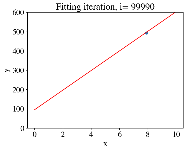
%%time
# Initial guess:
thetas[0,:] = [25,10]
alpha = 1

cnt = 0
for j in range(nrouter):
    for i in range(m-1):
        savethetas[cnt,:] = thetas[i,:]
        thetas[i+1,0] = thetas[i,0] - (alpha/m)  * (thetas[i,0] + thetas[i,1]*xshuf[i] - yshuf[i])            # note, we're using the non-vectorized version here
        thetas[i+1,1] = thetas[i,1] - (alpha/m)  * ((thetas[i,0] + thetas[i,1]*xshuf[i] - yshuf[i])*xshuf[i])

        # Note, this is not how one would compute the error in the real algorithm, but
        # we can use it just for plotting
        saveerrors[cnt] = mean_squared_error(thetas[i+1,0]+thetas[i+1,1]*xshuf,yshuf) /2
        cnt = cnt+1

        if (cnt<1000 and cnt % 100 == 0) or cnt % 10000 == 0 or cnt == nrouter*(m-1):
          my_plot(xshuf[i],yshuf[i],np.linspace(0,10,100),thetas[i+1,0] + thetas[i+1,1]*np.linspace(0,10,100),cnt,cnt == nrouter*(m-1))
    # if j % 10 == 0:
    #   print(j, "Starting over, now with initial guess:", thetas[m-1,:])
    thetas[0,:] = thetas[m-1,:] #

CPU times: user 51.2 s, sys: 95.9 ms, total: 51.3 s
Wall time: 54.6 s

Tet0 = savethetas[:,0]
Tet1 = savethetas[:,1]
print("Stochastic gradient descent error is", round(saveerrors[-2],2), \
      'with theta0, theta1',round(Tet0[-1],2) ,round(Tet1[-1],2), 'after', cnt, 'steps.')

fig = plt.figure(figsize=(10,10))
ax = fig.add_subplot(111, projection='3d')
ax.set_xlabel(r'$\theta_0$')
ax.set_ylabel(r'$\theta_1$')
ax.set_zlabel('Cost')

ax.scatter(thetas_batch[:,0], thetas_batch[:,1], error_batch/1000)
ax.plot(thetas_batch[:,0], thetas_batch[:,1], error_batch/1000)

ax.scatter(Tet0 , Tet1, saveerrors/1000, c='r', marker='o')
ax.plot(Tet0 , Tet1, saveerrors/1000, color='r')

ax.view_init(40, 0)
plt.show()

Stochastic gradient descent error is 108.56 with theta0, theta1 94.12 50.84 after 99990 steps.

In the figure above, the cost evolution of the batch gradient descent is also shown for comparison (in blue). Both follow a similar path, but the stochastic approach takes orders of magnitude more steps.

Clearly, stochastic gradient descent should only be used when the size of a data-set makes batch gradient descent impossible.

Here is the learning curve:

fig = plt.figure(figsize=(6,6))

plt.plot(range(len(saveerrors)), saveerrors,'r-')
plt.xlabel('Nr iterations')
plt.ylabel('Cost')
plt.title('Learning curve')
plt.ylim(0,1000)

Mini-Batch Gradient Descent

Sometimes an optimal approach for intermediate, but large, data-set can be a combination of batch and stochastic gradient descent method. The algorithm is implied by the name: instead of considering the full ‘batch’ of data in each fitting attempt, versus only 1 data point at a time in the stochastic approach, combine the best of both worlds and use a ‘mini-batch’. Basically, pick some mini-batch size, say \(b=10\). Then, for each update of the fitting parameters, only try and fit \(b\) of the points (e.g. going through the list of pre-randomized points).

%%time
batch = 10
nr_pass = 2
m = len(xshuf)
alpha_m = 0.01/batch

nrsteps = int(m/batch)
x_i = np.zeros([batch,2])
x_i[:,0] = 1
thetas = np.zeros([nrsteps+1,2])
errors = np.zeros(nrsteps*nr_pass)
thetas[0,:] = [25,10]

mb_iter=0
for j in range(nr_pass):
  for i in range(nrsteps):
    x_i[:,1] = xshuf[i*batch:(i+1)*batch]
    y_i = yshuf[i*batch:(i+1)*batch]
    hypothesis = x_i.dot(thetas[i,:])
    thetas[i+1,:] = thetas[i,:] - alpha_m * (hypothesis - y_i).dot(x_i)
    errors[mb_iter] = mean_squared_error(hypothesis,y_i) /2
    # Plotting:
    if (mb_iter<1000 and mb_iter % 10 == 0) or mb_iter == nrsteps-1:
     my_plot(np.squeeze(x_i[:,1]),y_i,np.linspace(0,10,100),thetas[i+1,0] + thetas[i+1,1]*np.linspace(0,10,100),mb_iter,mb_iter == nrsteps-1)

    mb_iter += 1
  thetas[0,:] = thetas[i+1,:]
  hypothesis = thetas[-1,0] + thetas[-1,1]*xshuf
  minibatcherror = mean_squared_error(hypothesis,yshuf) /2

CPU times: user 16.7 s, sys: 206 ms, total: 16.9 s
Wall time: 18.5 s

  print("Result after", j+1, "passes:", thetas[-1,:], "error:", minibatcherror, 'and total iterations:', mb_iter)

Result after 2 passes: [99.58621779 49.84960358] error: 105.04822636662745 and total iterations: 2000

If we look at the learning curve for the errors computed for individual batches, but plotted versus total number of iterations,

fig = plt.figure(figsize=(6,6))

plt.plot(range(len(errors)), errors,'r-')
plt.xlabel('Nr iterations')
plt.ylabel('Cost')
plt.title('Learning curve')
plt.ylim(0,1000)

we see that this looks far noisier than before. This is because the fitting results to small batches of 10 points can easily be higher/lower than the average across all data points.

Conclusion

This concludes the fairly comprehensive overview of some of the most widely used numerical regression algorithms. To see most clearly how they work, only linear regression of a single variable/feature was considered. In the next module, you will see that the extension to multivariate (many features) and non-linear functional relationships is surprisingly straightforward.

Even more interesting, these algorithms can also be applied to logistical regression in which the target \(y\) consists of 2 or more discrete categories, rather than a continuous numerical variable. [For example, some features might be hairlength \(x_1\), number of legs \(x_2\), average number of hours of sleeping \(x_3\), average running speed \(x_4\), and the target is \(y=\) cat or \(y=\) dog.]

Meaning that if you comprehend this notebook well, the hardest work is done and you already have a pretty thorough understanding of how many machine learning tools work.

---

✏️ Next up: Practice: Linear Regression

📖 Next module: Module 3: Multivariate Regression